クラスタリング・主成分分析・潜在モデル分析などを試してみる上で適切なデータセットはなんだろうと考えていました。アイリスのデータセットでさくっとやるのも良かったのですが、熟考した結果「動物」の分類だ!と閃きました 笑
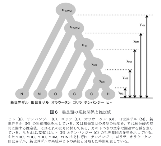
なぜ動物かというと以前ヒト・チンパンジー・ゴリラ・オラウータンが進化の過程でどう枝分かれしたかみたいなデータを見たときに印象に残っていたためです。
ヒトやチンパンジーをふくめて、すべての生物が共通の祖先から進化したという「進化論」の考え方をはじめて発表したのは、ダーウィン(Charles Robert Darwin、1809-1882)です。それから今日まで、発掘された骨の化石の形を分析したり、遺伝子をヒトやチンパンジーと比較したり、といったさまざまな研究が進み、共通祖先からどのようにヒトが進化してきたかも分かってきています。
引用: https://kids.gakken.co.jp/kagaku/kagaku110/science0043/
下記のような系統図です。
「類人猿分類公式マニュアル2.0 人間関係に必要な知恵はすべて類人猿に学んだ」という本の内容を抜粋するとDNAの一致率でいうと、ヒトと「チンパンジー」が98.8%、「ゴリラ」が97.7%、「オラウータン」が約96.4%のようです。(計算された時期や手法によって他の情報源と差異は発生するかも知れません。)
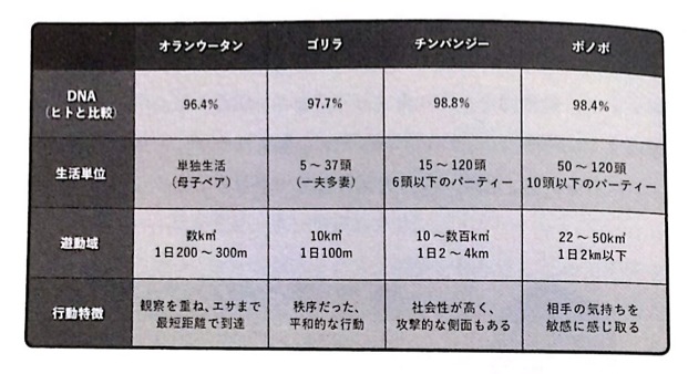
ヒトと最も近いのは系統図やDNAの一致率でいうとチンパンジーということになりますが、身体的特徴の類似度を考慮するとヒトはチンパンジーよりオラウータンに近いのではという意見もあるようです。
現存する人間に最も近い生物はチンパンジーではなくオランウータンだ。こう主張する最新の研究論文が議論を呼んでいる。 この結論は、オランウータンと人間が身体的に酷似していることに基づく...多くの科学者が引き合いに出すDNA鑑定は人間とチンパンジーのゲノムのごく一部しか調べていない...しかも、はるかに多くの動物が共有する古いDNAの形質がいくつも、人間とチンパンジーの類似点として挙げられている可能性がある。
引用: https://natgeo.nikkeibp.co.jp/nng/article/news/14/1352/
前置きが長くなってしまいましたが、動物の特徴量はグルーピング手法と相性がいいのではないかと思い探してみたらぴったりのデータセットがありました。
AwA2 (Animals with Attributes 2) のデータセットになります。
AwA2 (Animals with Attributes2)のデータセットとは
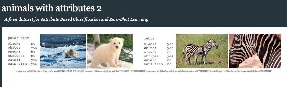
AwA2のデータセットは画像の著作権問題で利用制限中であるAwA (Animals with Attributes)の後継のデータセットになります。転移学習、特に属性ベースの分類とゼロショット学習のベンチマークとして利用されています。
50種類の動物(哺乳類)の画像が37322枚含まれており、各画像の特徴量は事前に抽出したものが用意されていました。また各クラスの属性情報(色やストライプの有無など全部で85カラム)も提供されています。
※ ちなみに画像は2016年にFlickrなどのパブリックソースから著作権フリーの画像を収集したそうです。
※ ゼロショット学習というワードが初めてでしたので調べてみると、学習データにはないがテストデータや未知のデータには存在するラベルを予測しようとするアプローチのようです。GMOさんのZero-shot learningの紹介:見たことがない画像やニュースを予測してみましたが事例も載っており分かりやすかったです。
観点が異なりますが、情報がないという点では何となく推薦システムのコールドスタート問題に通じるものがあるなと思いました。(詳しくはYahoo! JAPAN Tech Blogの機械学習の階層モデルの適用でコールドスタート問題に対処するが参考になります。)
人工知能/機械学習分野のゼロショット学習(Zero-shot Learning)とは、新しいクラス(分類問題の場合)やタスクを訓練データから事前に学習していなくても、推論時にその未知のクラスやタスクについての何らかの補助情報(説明テキストや属性情報、クラス間の類似性など)を訓練済みAIモデルに与えることで、柔軟に適切な分類や予測を行うための学習方法のことである。
引用: https://atmarkit.itmedia.co.jp/ait/articles/2307/27/news033.html
AwA2のデータセットの中身を確認する
それでは事前準備として、早速AwA2のデータセットをダウンロードして中身を確認してみたいと思います。
https://cvml.ista.ac.at/AwA2/ にアクセスし、AwA2-base.zipをダウンロードしてください。
Downloadsセクションにリンクがあります。もし画像も一緒に確認したい場合は13GBもありますが、AwA2-data.zipをダウンロードすると確認できます。
・Base package (32K) including the class/attribute table:AwA2-base.zip (same as for AwA1)
・Images in JPEG format and license files: AwA2-data.zip (13 GB!)
・(画像の特徴量は今回は使わない) Features extracted using an ILSVRC-pretrained ResNet101 (as used in [1]): AwA2-features.zip
動物クラスを確認
データセットに含まれる50種類の動物は下記になります。AwA2-base.zipもしくはAwA2-data.zipを解凍したフォルダ内のclasses.txtに記載されています。
犬や猫の具体的な種別も含まれているようですね。(英語の勉強にもなりました 笑)
| No. | 英名 | 日本語名 | 画像 | No. | 英名 | 日本語名 | 画像 |
|---|---|---|---|---|---|---|---|
| 1 | antelope | アンテロープ | 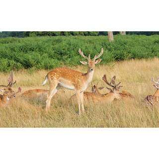 |
26 | hamster | ハムスター | 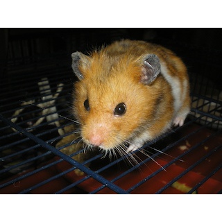 |
| 2 | grizzly+bear | グリズリーベア | 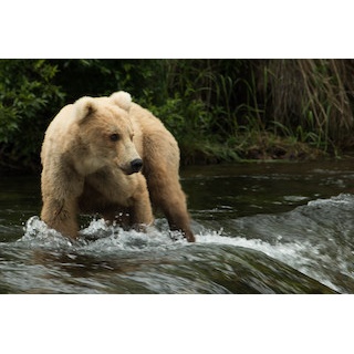 |
27 | squirrel | リス | 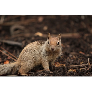 |
| 3 | killer+whale | シャチ | 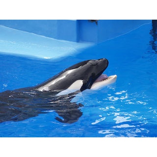 |
28 | rhinoceros | サイ | 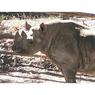 |
| 4 | beaver | ビーバー | 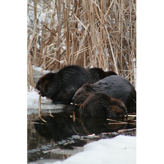 |
29 | rabbit | ウサギ | 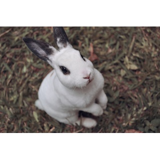 |
| 5 | dalmatian | ダルメシアン(犬) | 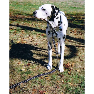 |
30 | bat | コウモリ | 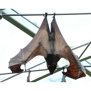 |
| 6 | persian+cat | ペルシャ(猫) | 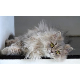 |
31 | giraffe | キリン | 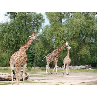 |
| 7 | horse | 馬 | 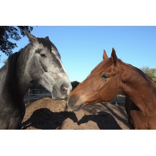 |
32 | wolf | オオカミ | 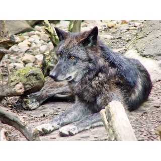 |
| 8 | german+shepherd | ジャーマンシェパード(犬) | 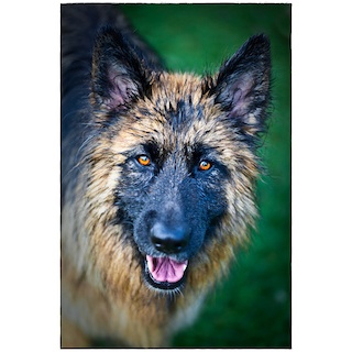 |
33 | chihuahua | チワワ(犬) | 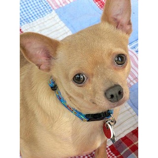 |
| 9 | blue+whale | シロナガスクジラ | 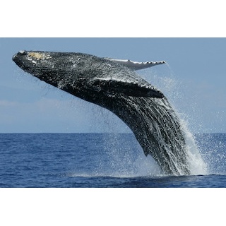 |
34 | rat | ラット(大型のネズミ) | 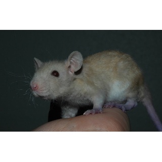 |
| 10 | siamese+cat | シャム(猫) | 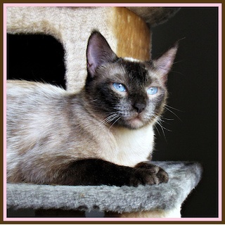 |
35 | weasel | イタチ | 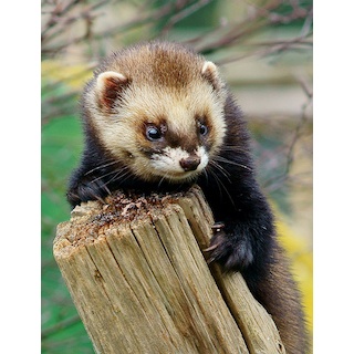 |
| 11 | skunk | スカンク | 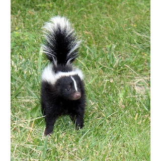 |
36 | otter | カワウソ | 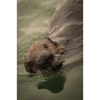 |
| 12 | mole | モグラ | 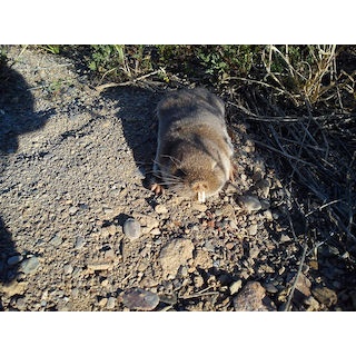 |
37 | buffalo | バッファロー | 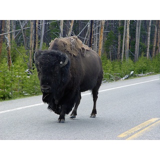 |
| 13 | tiger | トラ | 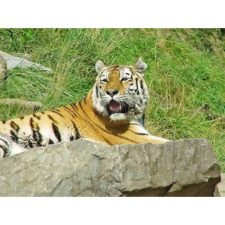 |
38 | zebra | シマウマ | 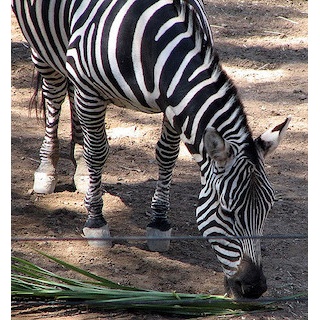 |
| 14 | hippopotamus | カバ | 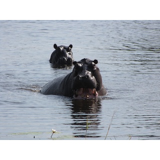 |
39 | giant+panda | ジャイアントパンダ | 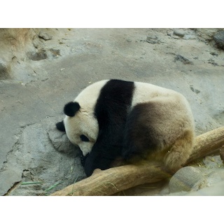 |
| 15 | leopard | ヒョウ | 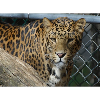 |
40 | deer | シカ | 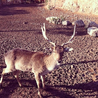 |
| 16 | moose | ヘラジカ | 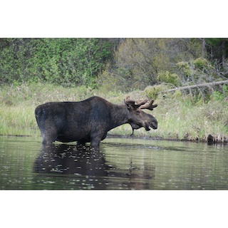 |
41 | bobcat | ボブキャット | 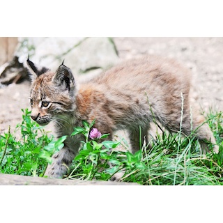 |
| 17 | spider+monkey | クモザル | 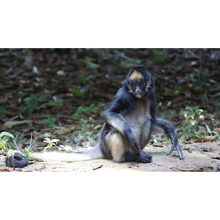 |
42 | pig | ブタ | 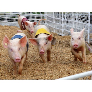 |
| 18 | humpback+whale | ザトウクジラ | 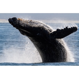 |
43 | lion | ライオン | 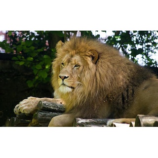 |
| 19 | elephant | 象 | 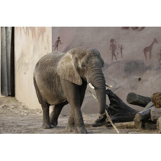 |
44 | mouse | マウス(小型のネズミ) | 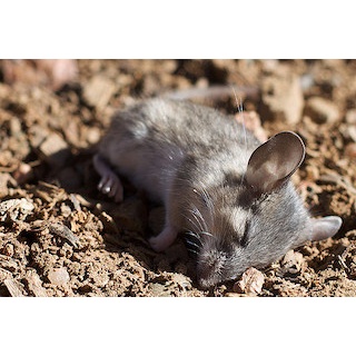 |
| 20 | gorilla | ゴリラ | 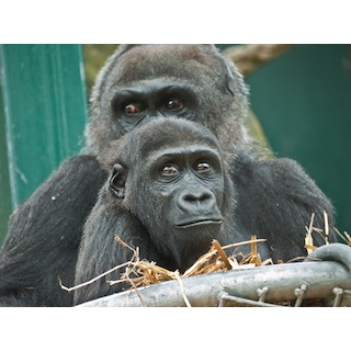 |
45 | polar+bear | ホッキョクグマ | 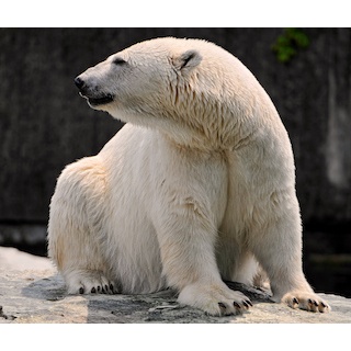 |
| 21 | ox | 雄牛 | 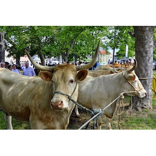 |
46 | collie | コリー(犬) | 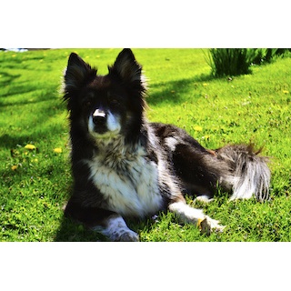 |
| 22 | fox | キツネ | 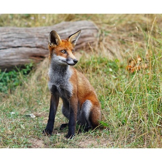 |
47 | walrus | セイウチ | 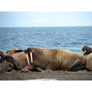 |
| 23 | sheep | 羊 | 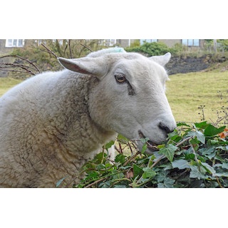 |
48 | raccoon | アライグマ | 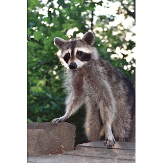 |
| 24 | seal | アザラシ | 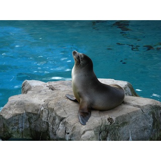 |
49 | cow | 雌牛 | 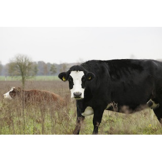 |
| 25 | chimpanzee | チンパンジー | 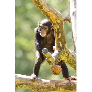 |
50 | dolphin | イルカ | 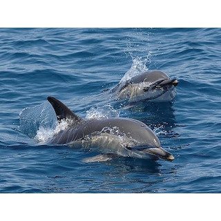 |
クラスタリングしたときにクジラやイルカは似たグループになりそうですね。またゴリラとクモザルは同じ様なカテゴリーに入るのでしょうか。
分析用に動物の属性情報のデータセット作成
まずは、50種類の動物 x 85属性情報を持ったデータフレームを作成しようと思います。
今回はK-Means, PCA, and Dendrogram on the Animals with Attributes Datasetを参考にしました。
下記の流れで分析を進めようと思います。 (参考にしたノートブックまんまですが 笑)
- 分析用データの作成
- 85次元を2次元で表現するため、主分析分析を実施
- 主成分分析の結果を活用し非階層クラスタリング(K-Means)でグルーピング
- 階層クラスタリングでグルーピング
分析用データの作成
BASE_DIR="/Users/hinomaruc/Desktop/blog/dataset/AwA2/Animals_with_Attributes2"
import pandas as pd
import os
from IPython.display import display, HTML

# 動物クラスの情報 (indexの情報として利用)
classes=pd.read_fwf(os.path.join(BASE_DIR,"classes.txt"), header=None)[1].values
print(classes)

# 属性情報名 (columnの情報として利用)
feature_names=pd.read_fwf(os.path.join(BASE_DIR,"predicates.txt"), header=None)[1].values
print(feature_names)

# 各動物クラスの属性情報 (データの中身)
features = pd.read_fwf(os.path.join(BASE_DIR,"predicate-matrix-continuous.txt"), header=None)
print(features.head())Out[0]['antelope' 'grizzly+bear' 'killer+whale' 'beaver' 'dalmatian' 'persian+cat' 'horse' 'german+shepherd' 'blue+whale' 'siamese+cat' 'skunk' 'mole' 'tiger' 'hippopotamus' 'leopard' 'moose' 'spider+monkey' 'humpback+whale' 'elephant' 'gorilla' 'ox' 'fox' 'sheep' 'seal' 'chimpanzee' 'hamster' 'squirrel' 'rhinoceros' 'rabbit' 'bat' 'giraffe' 'wolf' 'chihuahua' 'rat' 'weasel' 'otter' 'buffalo' 'zebra' 'giant+panda' 'deer' 'bobcat' 'pig' 'lion' 'mouse' 'polar+bear' 'collie' 'walrus' 'raccoon' 'cow' 'dolphin'] ['black' 'white' 'blue' 'brown' 'gray' 'orange' 'red' 'yellow' 'patches' 'spots' 'stripes' 'furry' 'hairless' 'toughskin' 'big' 'small' 'bulbous' 'lean' 'flippers' 'hands' 'hooves' 'pads' 'paws' 'longleg' 'longneck' 'tail' 'chewteeth' 'meatteeth' 'buckteeth' 'strainteeth' 'horns' 'claws' 'tusks' 'smelly' 'flys' 'hops' 'swims' 'tunnels' 'walks' 'fast' 'slow' 'strong' 'weak' 'muscle' 'bipedal' 'quadrapedal' 'active' 'inactive' 'nocturnal' 'hibernate' 'agility' 'fish' 'meat' 'plankton' 'vegetation' 'insects' 'forager' 'grazer' 'hunter' 'scavenger' 'skimmer' 'stalker' 'newworld' 'oldworld' 'arctic' 'coastal' 'desert' 'bush' 'plains' 'forest' 'fields' 'jungle' 'mountains' 'ocean' 'ground' 'water' 'tree' 'cave' 'fierce' 'timid' 'smart' 'group' 'solitary' 'nestspot' 'domestic'] 0 1 2 3 4 5 6 7 8 9 ... 75 \ 0 -1.00 -1.00 -1.0 -1.00 12.34 0.0 0.0 0.0 16.11 9.19 ... 0.00 1 39.25 1.39 0.0 74.14 3.75 0.0 0.0 0.0 1.25 0.00 ... 7.64 2 83.40 64.79 0.0 0.00 1.25 0.0 0.0 0.0 68.49 32.69 ... 79.49 3 19.38 0.00 0.0 87.81 7.50 0.0 0.0 0.0 0.00 7.50 ... 65.62 4 69.58 73.33 0.0 6.39 0.00 0.0 0.0 0.0 37.08 100.00 ... 1.25 76 77 78 79 80 81 82 83 84 0 0.00 1.23 10.49 39.24 17.57 50.59 2.35 9.70 8.38 1 9.79 53.14 61.80 12.50 24.00 3.12 58.64 20.14 11.39 2 0.00 0.00 38.27 9.77 52.03 24.94 15.77 13.41 15.42 3 0.00 0.00 3.75 31.88 41.88 23.44 31.88 33.44 13.12 4 6.25 0.00 9.38 31.67 53.26 24.44 29.38 11.25 72.71 [5 rows x 85 columns]
df_animals_attributes = pd.DataFrame(data=features.values,index=classes,columns=feature_names)
df_animals_attributes
      antelope  grizzly+bear    killer+whale    beaver  dalmatian
black   -1.00   39.25   83.40   19.38   69.58
white   -1.00   1.39    64.79   0.00    73.33
blue    -1.00   0.00    0.00    0.00    0.00
brown   -1.00   74.14   0.00    87.81   6.39
gray    12.34   3.75    1.25    7.50    0.00
...     ...     ...     ...     ...     ...
smart   17.57   24.00   52.03   41.88   53.26
group   50.59   3.12    24.94   23.44   24.44
solitary    2.35    58.64   15.77   31.88   29.38
nestspot    9.70    20.14   13.41   33.44   11.25
domestic    8.38    11.39   15.42   13.12   72.71

85 rows × 5 columns
作成したデータフレームの中身を確認
df_animals_attributes.info()Index: 50 entries, antelope to dolphin Data columns (total 85 columns): # Column Non-Null Count Dtype --- ------ -------------- ----- 0 black 50 non-null float64 1 white 50 non-null float64 2 blue 50 non-null float64 3 brown 50 non-null float64 4 gray 50 non-null float64 5 orange 50 non-null float64 6 red 50 non-null float64 7 yellow 50 non-null float64 8 patches 50 non-null float64 9 spots 50 non-null float64 10 stripes 50 non-null float64 11 furry 50 non-null float64 12 hairless 50 non-null float64 13 toughskin 50 non-null float64 14 big 50 non-null float64 15 small 50 non-null float64 16 bulbous 50 non-null float64 17 lean 50 non-null float64 18 flippers 50 non-null float64 19 hands 50 non-null float64 20 hooves 50 non-null float64 21 pads 50 non-null float64 22 paws 50 non-null float64 23 longleg 50 non-null float64 24 longneck 50 non-null float64 25 tail 50 non-null float64 26 chewteeth 50 non-null float64 27 meatteeth 50 non-null float64 28 buckteeth 50 non-null float64 29 strainteeth 50 non-null float64 30 horns 50 non-null float64 31 claws 50 non-null float64 32 tusks 50 non-null float64 33 smelly 50 non-null float64 34 flys 50 non-null float64 35 hops 50 non-null float64 36 swims 50 non-null float64 37 tunnels 50 non-null float64 38 walks 50 non-null float64 39 fast 50 non-null float64 40 slow 50 non-null float64 41 strong 50 non-null float64 42 weak 50 non-null float64 43 muscle 50 non-null float64 44 bipedal 50 non-null float64 45 quadrapedal 50 non-null float64 46 active 50 non-null float64 47 inactive 50 non-null float64 48 nocturnal 50 non-null float64 49 hibernate 50 non-null float64 50 agility 50 non-null float64 51 fish 50 non-null float64 52 meat 50 non-null float64 53 plankton 50 non-null float64 54 vegetation 50 non-null float64 55 insects 50 non-null float64 56 forager 50 non-null float64 57 grazer 50 non-null float64 58 hunter 50 non-null float64 59 scavenger 50 non-null float64 60 skimmer 50 non-null float64 61 stalker 50 non-null float64 62 newworld 50 non-null float64 63 oldworld 50 non-null float64 64 arctic 50 non-null float64 65 coastal 50 non-null float64 66 desert 50 non-null float64 67 bush 50 non-null float64 68 plains 50 non-null float64 69 forest 50 non-null float64 70 fields 50 non-null float64 71 jungle 50 non-null float64 72 mountains 50 non-null float64 73 ocean 50 non-null float64 74 ground 50 non-null float64 75 water 50 non-null float64 76 tree 50 non-null float64 77 cave 50 non-null float64 78 fierce 50 non-null float64 79 timid 50 non-null float64 80 smart 50 non-null float64 81 group 50 non-null float64 82 solitary 50 non-null float64 83 nestspot 50 non-null float64 84 domestic 50 non-null float64
とりあえずnullはなさそうですね。データ型も問題なさそうです。
df_animals_attributes.describe().transpose()
        count   mean    std     min     25%     50%     75%     max
black   50.0    35.3530     26.045034   -1.00   11.1500     34.335  47.3350     91.55
white   50.0    26.8552     27.883534   -1.00   4.4900  17.660  42.5250     95.62
blue    50.0    4.2134  11.683817   -1.00   0.0000  0.000   1.1700  67.08
brown   50.0    38.7088     25.864638   -1.00   15.7450     44.385  58.3775     91.20
gray    50.0    26.7472     22.947985   0.00    6.3150  24.115  39.3300     83.97
...     ...     ...     ...     ...     ...     ...     ...     ...
smart   50.0    33.6064     18.689228   8.75    17.7700     31.070  44.0900     84.36
group   50.0    31.0194     21.446729   0.00    13.5400     24.690  49.8625     80.60
solitary    50.0    25.8326     17.404436   0.00    8.9450  25.580  38.6700     59.47
nestspot    50.0    20.8992     10.667576   2.31    12.4975     18.990  28.1650     44.17
domestic    50.0    25.6106     26.516248   0.00    5.0350  12.950  44.7675     83.55
属性情報の数値がどう計算されているか気になったので調べてみた
データを見てみて数値情報の詳細が知りたかったので調べてみました。
README-attributes.txtに記載がありました。
Oshersonが収集したデータが元になっていて、それをKempが拡張したようです。
The numeric data was originally collected by Osherson et al. [1],
and extended by Kemp et al. [2].
[1] D. N. Osherson, J. Stern, O. Wilkie, M. Stob, and E. E.
Smith. Default probability. Cognitive Science, 15(2), 1991.
[2] C. Kemp, J. B. Tenenbaum, T. L. Griffiths, T. Yamada, and
N. Ueda. Learning systems of concepts with an infinite rela-
tional model. In AAAI, 2006.
Oshersonの記事はDefault Probabilityから確認することができました。
Kempの論文はLearning Systems of Concepts with an Infinite Relational Modelから確認することが出来ます。
Oshersonの記事を読む限り、まとめると下記になるようです。
- MITの学部生に対して広告を出して被験者を募集。参加者には報酬が支払われた。
- 被験者は、48の哺乳類の動物と85の属性のリストを確認し、各哺乳動物-属性のペアに非負の数値を割り当てるように指示された。
(今回のデータは50の哺乳類が存在するので後で拡張されたのかも知れません) - 数値は「属性と哺乳動物の間の関連性の相対的な強さを反映するべき」とされた。
(数値が高いほど関連性が高いということになりますね。) - すべての被験者の評価は線形変換によって0から1の範囲に正規化された。
- 各哺乳動物について、それを評価した8または9人の被験者の正規化されたスコアが平均された。
だいたい分かってきました。1つ前のセクションで確認したデータでは1より大きい数値も存在するので、-1は欠損、0~100の値を取り、数値が大きいほど対象の属性と関連性が高いということになりそうです。
※ -1が欠損値だと理解したのは、README-attributes.txt内に記載があったためです。
Missing values in the numeric table are marked by -1
理解が進んだので、数件のサンプルを覗いてみます。
数件ピックアップして確認
特徴が想像しやすく分かりやすい哺乳動物を選択しデータの中身を確認してみます。
from IPython.display import display, HTML
HTML(df_animals_attributes.loc[['killer+whale', 'zebra', 'elephant']].transpose().to_html())| attribute | killer+whale | zebra | elephant |
|---|---|---|---|
| black | 83.40 | 85.04 | 2.50 |
| white | 64.79 | 85.04 | 3.75 |
| blue | 0.00 | 0.00 | 0.00 |
| brown | 0.00 | 0.00 | 15.23 |
| gray | 1.25 | 0.00 | 83.97 |
| orange | 0.00 | 0.00 | 0.00 |
| red | 0.00 | 0.00 | 0.00 |
| yellow | 0.00 | 0.00 | 0.00 |
| patches | 68.49 | 0.00 | 0.00 |
| spots | 32.69 | 0.00 | 1.25 |
| stripes | 0.00 | 98.86 | 0.00 |
| furry | 1.25 | 36.40 | 1.14 |
| hairless | 70.62 | 7.69 | 68.27 |
| toughskin | 57.04 | 20.80 | 77.62 |
| big | 90.85 | 48.82 | 85.48 |
| small | 1.25 | 8.18 | 1.25 |
| bulbous | 61.87 | 11.88 | 48.52 |
| lean | 22.68 | 38.74 | 1.25 |
| flippers | 79.94 | 0.00 | 0.00 |
| hands | 0.00 | 0.00 | 0.00 |
| hooves | 0.00 | 76.45 | 10.60 |
| pads | 0.00 | 0.00 | 17.10 |
| paws | 0.00 | 0.00 | 5.08 |
| longleg | 0.00 | 39.02 | 39.14 |
| longneck | 1.25 | 21.88 | 1.25 |
| tail | 41.67 | 61.43 | 51.97 |
| chewteeth | 12.50 | 64.72 | 38.16 |
| meatteeth | 45.15 | 0.00 | 0.00 |
| buckteeth | 5.00 | 14.38 | 11.25 |
| strainteeth | 30.22 | 6.25 | 0.00 |
| horns | 0.00 | 0.00 | 1.14 |
| claws | 0.00 | 0.00 | 0.00 |
| tusks | 0.00 | 0.00 | 70.47 |
| smelly | 7.50 | 9.55 | 49.67 |
| flys | 1.25 | 0.00 | 3.75 |
| hops | 0.00 | 4.17 | 0.00 |
| swims | 91.45 | 0.00 | 0.00 |
| tunnels | 0.00 | 0.00 | 0.00 |
| walks | 0.00 | 77.61 | 66.19 |
| fast | 57.37 | 70.85 | 3.75 |
| slow | 5.14 | 1.25 | 63.03 |
| strong | 63.35 | 29.85 | 67.45 |
| weak | 1.25 | 16.25 | 0.00 |
| muscle | 10.45 | 38.76 | 25.56 |
| bipedal | 0.00 | 0.00 | 0.00 |
| quadrapedal | 0.00 | 89.00 | 70.61 |
| active | 27.29 | 42.51 | 6.48 |
| inactive | 13.23 | 20.00 | 53.62 |
| nocturnal | 8.75 | 0.00 | 7.50 |
| hibernate | 0.00 | 0.00 | 0.00 |
| agility | 27.80 | 29.52 | 5.78 |
| fish | 66.75 | 0.00 | 0.00 |
| meat | 21.81 | 5.14 | 5.68 |
| plankton | 32.86 | 0.00 | 0.00 |
| vegetation | 3.75 | 74.30 | 55.85 |
| insects | 0.00 | 0.00 | 1.25 |
| forager | 10.89 | 32.08 | 8.06 |
| grazer | 0.00 | 78.67 | 43.83 |
| hunter | 57.87 | 4.17 | 3.75 |
| scavenger | 6.61 | 0.00 | 2.50 |
| skimmer | 20.36 | 0.00 | 0.00 |
| stalker | 15.00 | 0.00 | 0.00 |
| newworld | 16.25 | 5.42 | 4.53 |
| oldworld | 12.50 | 90.92 | 84.56 |
| arctic | 24.51 | 0.00 | 0.00 |
| coastal | 30.11 | 0.00 | 0.00 |
| desert | 0.00 | 0.00 | 8.75 |
| bush | 0.00 | 41.53 | 36.91 |
| plains | 0.00 | 58.91 | 14.11 |
| forest | 0.00 | 8.75 | 7.58 |
| fields | 0.00 | 29.09 | 16.10 |
| jungle | 0.00 | 10.00 | 36.33 |
| mountains | 0.00 | 10.00 | 0.00 |
| ocean | 88.28 | 0.00 | 0.00 |
| ground | 0.00 | 82.75 | 66.81 |
| water | 79.49 | 0.00 | 1.25 |
| tree | 0.00 | 0.00 | 0.00 |
| cave | 0.00 | 0.00 | 0.00 |
| fierce | 38.27 | 0.00 | 20.63 |
| timid | 9.77 | 53.25 | 39.36 |
| smart | 52.03 | 22.63 | 22.81 |
| group | 24.94 | 80.60 | 49.87 |
| solitary | 15.77 | 1.25 | 6.25 |
| nestspot | 13.41 | 19.09 | 12.29 |
| domestic | 15.42 | 9.94 | 6.88 |
特徴的な属性を抜粋してみました。
数値が高いほどその動物の特徴を色濃く表現出来ていそうですね。
| attribute | killer+whale | zebra | elephant |
|---|---|---|---|
| black(黒) | 83.40 | 85.04 | 2.50 |
| white(白) | 64.79 | 85.04 | 3.75 |
| gray(灰色) | 1.25 | 0.00 | 83.97 |
| patches(斑模様?) | 68.49 | 0.00 | 0.00 |
| swims(泳ぐ) | 91.45 | 0.00 | 0.00 |
| smart(賢い) | 52.03 | 22.63 | 22.81 |
| group(群れ) | 24.94 | 80.60 | 49.87 |
| newworld(南北アメリカおよびオーストラリアに存在) | 16.25 | 5.42 | 4.53 |
| oldworld(アジア、ヨーロッパ、アフリカなどに存在) | 12.50 | 90.92 | 84.56 |
属性名ごとに一番数値が低い動物と高い動物を確認
属性名が短く省略されているので、属性ごとに一番数値が低い動物と一番数値が高い動物の一覧を作成してどのような意味か推定しようと思います。
一部Oshersonの記事にも省略されていない属性の意味が記載されているので、そちらも参考にしながらまとめてみます。
# 各列ごとに最小値、最小値のインデックス、最大値、最大値のインデックスを計算
min_values = df_animals_attributes[df_animals_attributes > 0].min()
min_indexes = df_animals_attributes[df_animals_attributes > 0].idxmin()
max_values = df_animals_attributes.max()
max_indexes = df_animals_attributes.idxmax()

# 新しいデータフレームを作成して情報をまとめる
summary_df = pd.DataFrame({
    '最小値': min_values,
    '最小値のindex': min_indexes,
    '最大値': max_values,
    '最大値のindex': max_indexes
})

# 描画
HTML(summary_df.to_html())※ 見やすいようにアウトプットは加工しています。
| 最小値 | 最小値のindex | 最大値 | 最大値のindex | 最小値 | 最小値のindex | 最大値 | 最大値のindex | ||
|---|---|---|---|---|---|---|---|---|---|
| black | 1.88 | lion | 91.55 | bat | muscle | 0.62 | mouse | 82.34 | tiger |
| white | 1.25 | lion | 95.62 | polar+bear | bipedal | 0.62 | collie | 68.80 | gorilla |
| blue | 1.56 | seal | 67.08 | blue+whale | quadrapedal | 4.80 | dolphin | 89.00 | zebra |
| brown | 0.33 | dolphin | 91.20 | moose | active | 2.64 | rhinoceros | 77.80 | chimpanzee |
| gray | 1.25 | killer+whale | 83.97 | elephant | inactive | 1.11 | horse | 53.62 | elephant |
| orange | 1.49 | cow | 72.91 | tiger | nocturnal | 0.62 | dolphin | 98.86 | bat |
| red | 0.12 | chihuahua | 40.89 | fox | hibernate | 1.11 | horse | 86.14 | grizzly+bear |
| yellow | 0.16 | dolphin | 48.43 | giraffe | agility | 3.52 | pig | 88.33 | spider+monkey |
| patches | 0.62 | chimpanzee | 84.95 | giant+panda | fish | 0.62 | spider+monkey | 83.33 | otter |
| spots | 0.80 | dolphin | 100.00 | dalmatian | meat | 0.30 | cow | 86.97 | tiger |
| stripes | 1.25 | leopard | 98.86 | zebra | plankton | 3.12 | beaver | 82.30 | humpback+whale |
| furry | 0.62 | dolphin | 90.19 | persian+cat | vegetation | 1.25 | leopard | 78.06 | moose |
| hairless | 0.46 | chimpanzee | 73.27 | dolphin | insects | 0.62 | lion | 46.43 | bat |
| toughskin | 0.62 | chihuahua | 77.62 | elephant | forager | 1.25 | otter | 77.01 | squirrel |
| big | 1.25 | mole | 94.60 | humpback+whale | grazer | 0.25 | walrus | 78.67 | zebra |
| small | 1.25 | killer+whale | 86.05 | chihuahua | hunter | 0.62 | mole | 84.93 | tiger |
| bulbous | 0.62 | chihuahua | 82.08 | walrus | scavenger | 0.72 | cow | 60.85 | rat |
| lean | 1.25 | elephant | 73.48 | leopard | skimmer | 1.12 | grizzly+bear | 50.11 | humpback+whale |
| flippers | 4.38 | beaver | 86.44 | dolphin | stalker | 0.62 | mouse | 87.22 | tiger |
| hands | 1.25 | walrus | 77.77 | chimpanzee | newworld | 2.64 | rhinoceros | 82.33 | moose |
| hooves | 10.60 | elephant | 86.32 | horse | oldworld | 3.95 | grizzly+bear | 90.92 | zebra |
| pads | 0.56 | giraffe | 42.44 | persian+cat | arctic | 1.11 | siamese+cat | 96.88 | polar+bear |
| paws | 1.25 | gorilla | 76.17 | collie | coastal | 1.25 | dalmatian | 59.15 | seal |
| longleg | 1.25 | pig | 84.01 | giraffe | desert | 0.31 | cow | 22.50 | lion |
| longneck | 1.25 | killer+whale | 96.71 | giraffe | bush | 2.50 | german+shepherd | 65.09 | chimpanzee |
| tail | 5.39 | buffalo | 86.56 | beaver | plains | 1.25 | spider+monkey | 68.84 | buffalo |
| chewteeth | 5.92 | bobcat | 64.72 | zebra | forest | 1.25 | sheep | 77.40 | grizzly+bear |
| meatteeth | 0.62 | buffalo | 85.88 | tiger | fields | 1.25 | dalmatian | 70.14 | horse |
| buckteeth | 2.47 | antelope | 83.12 | beaver | jungle | 0.25 | rabbit | 91.98 | chimpanzee |
| strainteeth | 0.19 | cow | 69.32 | blue+whale | mountains | 0.62 | mole | 67.19 | moose |
| horns | 1.14 | elephant | 93.02 | moose | ocean | 35.00 | otter | 89.36 | humpback+whale |
| claws | 3.75 | seal | 75.05 | tiger | ground | 10.00 | otter | 84.48 | rat |
| tusks | 1.25 | ox | 90.74 | walrus | water | 0.55 | cow | 89.95 | humpback+whale |
| smelly | 1.95 | squirrel | 100.00 | skunk | tree | 1.25 | fox | 81.36 | chimpanzee |
| flys | 0.82 | dolphin | 95.90 | bat | cave | 0.32 | cow | 80.62 | bat |
| hops | 1.14 | raccoon | 87.59 | rabbit | fierce | 1.11 | giraffe | 83.81 | tiger |
| swims | 0.25 | lion | 91.45 | killer+whale | timid | 2.27 | raccoon | 67.49 | deer |
| tunnels | 0.19 | cow | 77.61 | mole | smart | 8.75 | hippopotamus | 84.36 | chimpanzee |
| walks | 2.50 | bat | 78.90 | ox | group | 0.62 | collie | 80.60 | zebra |
| fast | 2.50 | hippopotamus | 85.26 | leopard | solitary | 1.25 | zebra | 59.47 | bobcat |
| slow | 1.11 | horse | 68.69 | hippopotamus | nestspot | 2.31 | hippopotamus | 44.17 | gorilla |
| strong | 1.25 | mole | 88.78 | ox | domestic | 2.31 | buffalo | 83.55 | siamese+cat |
| weak | 1.11 | horse | 61.36 | chihuahua |
属性名の意味一覧 (推測)
前セクションの結果を省みて、各属性の意味をまとめてみました。
| 属性名 | 日本語訳 | 属性名 | 日本語訳 |
|---|---|---|---|
| black | 黒い | muscle | 筋肉質な |
| white | 白い | bipedal | 二足歩行可能な |
| blue | 青い | quadrapedal | 四足歩行可能な |
| brown | 茶色い | active | 活動的な |
| gray | 灰色 | inactive | 非活動的な |
| orange | オレンジ色 | nocturnal | 夜行性 |
| red | 赤い | hibernate | 冬眠する |
| yellow | 黄色い | agility | すばしっこい |
| patches | 斑ら模様な | fish | 魚を食べる |
| spots | 点々模様な | meat | 肉を食べる |
| stripes | ストライプ模様な | plankton | プランクトンを食べる |
| furry | 毛皮でおおわれた | vegetation | 草を食べる |
| hairless | 毛がない | insects | 虫を食べる |
| toughskin | 頑丈な | forager | 食物を探し回り収集する |
| big | 大きな | grazer | 草食動物 |
| small | 小さな | hunter | 狩猟者(肉食動物?) |
| bulbous | 太っていて丸い感じ | scavenger | 腐肉食(死骸などを食べる) |
| lean | 痩せた | skimmer | (水面上を)すくい取る |
| flippers | ヒレがある | stalker | 追いかけてくる |
| hands | 手がある | newworld | 南北アメリカおよびオーストラリアに生息(おそらく南北アメリカがメイン) |
| hooves | 蹄(ひづめ)がある | oldworld | アジア、ヨーロッパ、アフリカなどに生息(おそらくアフリカがメイン) |
| pads | 足裏が柔らかい(パッドがある) | arctic | 北極圏に生息 |
| paws | 肉球がある | coastal | 沿岸・海岸地帯に生息 |
| longleg | 足が長い | desert | 砂漠地帯に生息 |
| longneck | 首が長い | bush | 低木・灌木が生えている地帯に生息 |
| tail | 尻尾がある | plains | 平原・平原地帯に生息 |
| chewteeth | 噛むのに適した臼歯を持っている | forest | 森林地帯に生息 |
| meatteeth | 肉を食べるのに適した歯を持っている(犬歯?) | fields | 野原・畑地帯に生息 |
| buckteeth | 出っ歯がある | jungle | ジャングルに生息 |
| strainteeth | (自信ないが)繊維状の歯がある | mountains | 山に生息 |
| horns | 角がある | ocean | 海で生活 |
| claws | 爪がある | ground | 地面で生活 |
| tusks | 牙がある | water | 水中で生活 |
| smelly | 匂いがする(臭い) | tree | 木で生活 |
| flys | 飛ぶ(移動手段) | cave | 洞窟で生活 |
| hops | 跳ねる(移動手段) | fierce | 獰猛な |
| swims | 泳ぐ(移動手段) | timid | 臆病な |
| tunnels | 穴を掘る(移動手段) | smart | かしこい |
| walks | 歩く(移動手段) | group | 群れる |
| fast | 速い | solitary | 孤独な |
| slow | 遅い | nestspot | 巣作りをする(縄張りがあるとか?) |
| strong | 強い | domestic | 家庭で飼われる |
| weak | 弱い |
PCAで次元削減を試してみる (2次元)
さてデータの理解も進んだので、まずは主成分分析を試してみたいと思います。85次元の情報を扱うのは大変なので2次元で表現させてみたいと思います。
import numpy as np
import pandas as pd
import seaborn as sns
# 描画設定
sns.set_style("whitegrid")
from matplotlib import rcParams
rcParams['font.family'] = 'Hiragino Sans' # Macの場合
#rcParams['font.family'] = 'Meiryo' # Windowsの場合
#rcParams['font.family'] = 'VL PGothic' # Linuxの場合
rcParams['xtick.labelsize'] = 12       # x軸のラベルのフォントサイズ
rcParams['ytick.labelsize'] = 12       # y軸のラベルのフォントサイズ
rcParams['axes.labelsize'] = 18        # ラベルのフォントとサイズ
rcParams['figure.figsize'] = 18,8 # 画像サイズの変更(inch)from sklearn.decomposition import PCA
X=df_animals_attributes.values
pca = PCA(n_components=2)
X_pca = pca.fit(X).transform(X)
print("Before: X.shape",X.shape)
print("After: X_pca.shape",X_pca.shape)Before: X.shape (50, 85) After: X_pca.shape (50, 2)
無事85次元の情報量を2次元で表現できたようです。これは描画するときに役立ちます。3次元データにして3Dで描画するのもありかも?
import matplotlib.pyplot as plt
from adjustText import adjust_text

# 主成分のプロット
plt.scatter(X_pca[:, 0], X_pca[:, 1])
plt.xlabel('Principal Component 1')
plt.ylabel('Principal Component 2')
plt.title('PCA Results')

texts = []
# 各プロットにクラス名を追加。ラベル配置調整用にリストにも追加。
for idx,aclass in enumerate(classes):
    texts.append(plt.text(X_pca[idx, 0], X_pca[idx, 1], aclass, fontsize=12, ha='center', va='bottom'))

# ラベル位置の調整 (adjustTextというツールを使っています。pip install adjustTextで事前にインストールが必要)
adjust_text(texts, force_points=0.2, force_text=0.2, expand_points=(1, 1))

plt.show()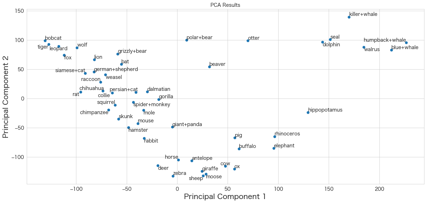
クジラ系や猫・犬などは似たような位置に存在していることが分かりますね。雄牛・雌牛も隣同士のようです。ほぼ似たような特性なのでしょうね。
一方でグリズリーベアとホッキョクグマはPCAの結果だと距離が少し離れているように見えます。森の中で生活しているか海の近くで生活しているかの違いが出ているのでしょうか?
気になるのでクマだけ個別にデータを確認しておこうと思います。
from IPython.display import display, HTML
HTML(df_animals_attributes.loc[['grizzly+bear', 'polar+bear']].transpose().to_html())
      grizzly+bear  polar+bear
black     39.25     10.00
white      1.39     95.62
swims      2.50     39.17
oldworld   3.95     31.25
arctic     6.65     96.88
coastal    2.78     48.96
mountains  43.85    1.25
一部抜粋しています。上記らへんで違いが出ているのかも知れないと思いました。
PCAで次元削減を試してみる (3次元)
せっかくなので3次元バージョンも試してみたいと思います。
描画にはplotlyを利用しました。(matplotlibだとクラス名が全て重なってしまってよく分からないグラフになってしまったので、、)
from sklearn.decomposition import PCA

pca = PCA(n_components=3)
X_pca3d = pca.fit(X).transform(X)

print("Before: X.shape",X.shape)
print("After: X_pca3d.shape",X_pca3d.shape)

import plotly.express as px

# データフレームを作成
import pandas as pd

df = pd.DataFrame({'PC1': X_pca3d[:, 0], 'PC2': X_pca3d[:, 1], 'PC3': X_pca3d[:, 2], 'Class': classes})

# 3D Scatter plotを作成
fig = px.scatter_3d(df, x='PC1', y='PC2', z='PC3', color='Class', text='Class', opacity=0.7)

fig.update_layout(
    scene=dict(
        xaxis_title='Principal Component 1',
        yaxis_title='Principal Component 2',
        zaxis_title='Principal Component 3',
    ),
    title='PCA Results in 3D',
    width=800,  # Set the width of the figure
    height=600, # Set the height of the figure
)

# ラベルの位置調整
fig.update_traces(textposition='bottom center', selector=dict(mode='markers+text'))

fig.show()Before: X.shape (50, 85)
After: X_pca3d.shape (50, 3)
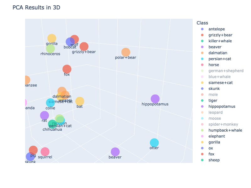
グリズリーベアとホッキョクグマは3Dで見ても同じような距離感ですね 笑
K-Meansでクラスタリングを試してみる
非階層クラスタリングです。
85カラムの中から、自分で分類に使いたい特徴量を選択しK-Meansにかけてみるという方法もあるかと思いますが、今回はサンプルに倣ってPCAの結果(2次元に圧縮したもの)をそのままK-Meansアルゴリズムでクラスタリングしてみようと思います。
from sklearn.cluster import KMeans

# とりあえず8つに分けてみる。エルボー法とかで最適な分割数を求めてもよし
n_clusters = 8

# random_stateを設定しないと毎回結果が変わるので再現性を重視する場合は注意
kmeans = KMeans(n_clusters=n_clusters,n_init="auto",random_state=1111)

# fitする
clusters = kmeans.fit_predict(X_pca)

# Define a color map for clusters
cluster_colors = plt.cm.viridis(np.linspace(0, 1, n_clusters))

# Visualize the clusters in 2D PCA space
plt.scatter(X_pca[:, 0], X_pca[:, 1], c=clusters, cmap='viridis', s=50)
plt.title('PCA Results with Clusters')
plt.xlabel('Principal Component 1')
plt.ylabel('Principal Component 2')

texts = []
# 各プロットにクラス名を追加。ラベル配置調整用にリストにも追加。
for idx,aclass in enumerate(classes):
    texts.append(plt.text(X_pca[idx, 0], X_pca[idx, 1], aclass, fontsize=12, ha='center', va='bottom'))

# ラベル位置の調整 (adjustTextというツールを使っています。pip install adjustTextで事前にインストールが必要)
adjust_text(texts, force_points=0.2, force_text=0.2, expand_points=(1, 1))

# Create a custom legend
legend_labels = [f'Cluster {i}' for i in range(n_clusters)]
legend_handles = [plt.Line2D([0], [0], marker='o', color='w', markerfacecolor=cluster_colors[i], markersize=10, label=legend_labels[i]) for i in range(n_clusters)]

plt.legend(handles=legend_handles, title='Cluster Numbers', loc='lower right')

plt.show()
# データブレームにクラスタ番号追加
df_animals_attributes['Cluster'] = clusters
HTML(df_animals_attributes.groupby('Cluster').mean().transpose().to_html())※ 一部抜粋です。
Cluster 0 1 2 3 4 5 6 7
black 40.290 38.558333 25.378571 36.929091 4.77 25.396667 29.740000 48.355000
big 20.266 71.183333 54.491429 37.867273 79.48 34.540000 73.723333 13.088333
swims 3.125 78.558333 0.532857 3.027273 40.37 66.076667 0.701667 1.620000
hunter 11.383 24.618333 4.511429 60.828182 3.75 30.996667 2.035000 1.840000
クラスタごとの平均値を確認すると特色が浮き彫り出てきます。通常ここでクラスタごとに名前をつける作業が発生します (ネーミングのセンスが問われます 笑)
クラスタ1は海系の動物かなとかクラスタ3は肉食動物系かなとか考える時間になります。
ネーミング後に実業務では、クラスタの特色ごとに施策を考えて実行して、ランダムにやった場合と比べてどれくらい効果があるかなど確認していくことが多いかも知れません。
階層型クラスタリングを試す
デンドログラムを描画してみようと思います。
from scipy.cluster.hierarchy import dendrogram, linkage,fcluster
cluster_link = linkage(X, method='ward');
dendrogram(cluster_link,labels=classes)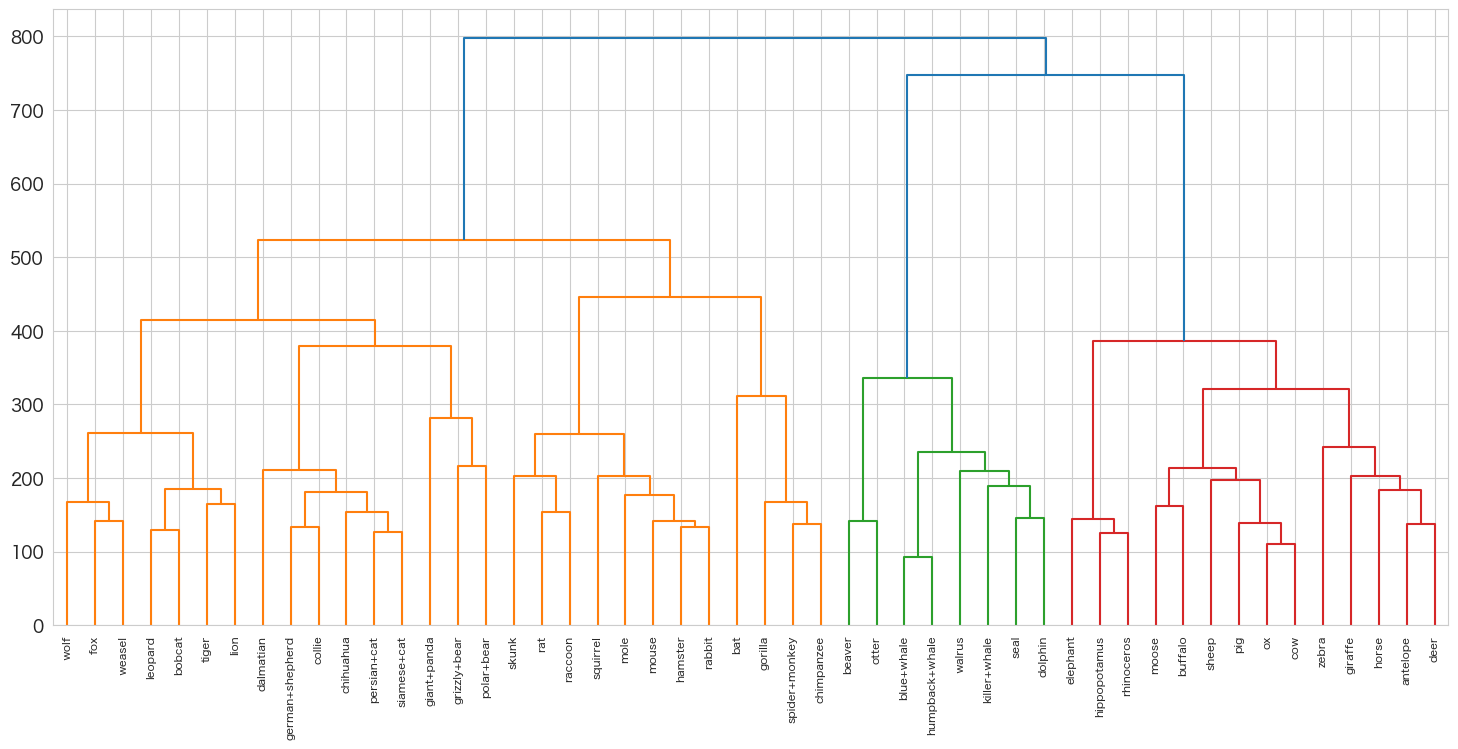
美しいですね。自分の好みの集団を作成することが出来ますね。
データ量が多くなると確認が大変なので、非階層クラスタリングの方が向いているデータセットもあるかと思いますか、今回は50レコードが対象なので階層型に向いていそうですね。
系統図みたいに直感的に似ている動物が近くいそうですね。
ゴリラ・クモザル・チンパンジーが近くに存在するらしく想定通りになりました。
ビーバーとカワウソも見た目で言うと近くにいるのは分かりますね。
今回投入変数として「見た目」・「生息場所」・「移動手段」・「何を食べるか」など全てを使いましたが、見た目でも色系は除くなどすればまた結果は変わってきそうですね。
何を目的として分類するのかを考えた上で投入変数を選択することが大事だと感じました。
scipyにはf(lat)clusterというメソッドも用意されていて、特定の条件でクラスタ番号を自動的に振り分けるといったことも可能でした。
※ 閾値の値を設定するのが大変でしたが、、
下記のような感じで使います。
fcluster(cluster_link,t=200, criterion='distance')
array([21, 5, 16, 14, 4, 3, 21, 3, 15, 3, 9, 10, 2, 18, 2, 19, 12,
15, 18, 12, 20, 1, 20, 16, 12, 10, 11, 18, 10, 13, 22, 1, 3, 8,
1, 14, 19, 23, 7, 21, 2, 20, 2, 10, 6, 3, 17, 8, 20, 16],
dtype=int32)
まとめ
今回はデータセットの中身の理解に時間がかかりました。ただクラスタリングなどの分類用のデータセットとしては分かりやすいしいいサンプルになりそうです。
次はソフトクラスタリングと潜在クラス分析あたりをやってみようと思います。
ライブラリのバージョンまとめは下記
pandas==2.0.3
numpy==1.24.4
scikit-learn==1.3.0
scipy==1.10.1
plotly==5.17.0
matplotlib==3.7.3
adjustText==0.8