前回はRandom Forestで分類モデルを作成しました。
精度はデフォルト設定のままだったのか、0.73205でした。
暫定1位はロジスティック回帰CVで作成してモデルで、Kaggleの精度は0.76794です。
今回はお待ちかねのXGBoostを試してみようと思います。
よくコンペで利用されるアルゴリズムですね。
XGBoost is an optimized distributed gradient boosting library designed to be highly efficient, flexible and portable. 引用: https://xgboost.readthedocs.io/en/stable/
XGBoostは最適化された分散型勾配ブースティングで高効率かつ柔軟でポータブルになるよう設計されたライブラリのようです。
ここでいうポータブルはどういう意味なんでしょうね。おそらく軽量・移植可能・独立したパッケージという意味で使われているのかも知れません。
勾配ブースティングとは下記の意味のようです。
弱い予測モデル weak prediction model(通常は決定木)のアンサンブルの形で予測モデルを生成する:https://ja.wikipedia.org/wiki/勾配ブースティング
それでは試してみます。XGBoost回帰(XGBRegressor)ではなくXGBoost分類(XGBClassifier)を使います。
評価指標
タイタニックのデータセットは生存有無を正確に予測できた乗客の割合(Accuracy)を評価指標としています。
分析用データの準備
事前に欠損値処理や特徴量エンジニアリングを実施してデータをエクスポートしています。
本記事と同じ結果にするためには事前に下記記事を確認してデータを用意してください。
学習データと評価データの読み込み
import pandas as pd
import numpy as np
# タイタニックデータセットの学習用データと評価用データの読み込み
df_train = pd.read_csv("/Users/hinomaruc/Desktop/notebooks/titanic/titanic_train.csv")
df_eval = pd.read_csv("/Users/hinomaruc/Desktop/notebooks/titanic/titanic_eval.csv")
概要確認
# 概要確認
df_train.info()
    RangeIndex: 891 entries, 0 to 890
    Data columns (total 22 columns):
     #   Column         Non-Null Count  Dtype
    ---  ------         --------------  -----
     0   PassengerId    891 non-null    int64
     1   Survived       891 non-null    int64
     2   Pclass         891 non-null    int64
     3   Name           891 non-null    object
     4   Sex            891 non-null    object
     5   Age            891 non-null    float64
     6   SibSp          891 non-null    int64
     7   Parch          891 non-null    int64
     8   Ticket         891 non-null    object
     9   Fare           891 non-null    float64
     10  Cabin          204 non-null    object
     11  Embarked       891 non-null    object
     12  FamilyCnt      891 non-null    int64
     13  SameTicketCnt  891 non-null    int64
     14  Pclass_str_1   891 non-null    float64
     15  Pclass_str_2   891 non-null    float64
     16  Pclass_str_3   891 non-null    float64
     17  Sex_female     891 non-null    float64
     18  Sex_male       891 non-null    float64
     19  Embarked_C     891 non-null    float64
     20  Embarked_Q     891 non-null    float64
     21  Embarked_S     891 non-null    float64
    dtypes: float64(10), int64(7), object(5)
    memory usage: 153.3+ KB
# 概要確認
df_eval.info()
    RangeIndex: 418 entries, 0 to 417
    Data columns (total 21 columns):
     #   Column         Non-Null Count  Dtype
    ---  ------         --------------  -----
     0   PassengerId    418 non-null    int64
     1   Pclass         418 non-null    int64
     2   Name           418 non-null    object
     3   Sex            418 non-null    object
     4   Age            418 non-null    float64
     5   SibSp          418 non-null    int64
     6   Parch          418 non-null    int64
     7   Ticket         418 non-null    object
     8   Fare           418 non-null    float64
     9   Cabin          91 non-null     object
     10  Embarked       418 non-null    object
     11  Pclass_str_1   418 non-null    float64
     12  Pclass_str_2   418 non-null    float64
     13  Pclass_str_3   418 non-null    float64
     14  Sex_female     418 non-null    float64
     15  Sex_male       418 non-null    float64
     16  Embarked_C     418 non-null    float64
     17  Embarked_Q     418 non-null    float64
     18  Embarked_S     418 non-null    float64
     19  FamilyCnt      418 non-null    int64
     20  SameTicketCnt  418 non-null    int64
    dtypes: float64(10), int64(6), object(5)
    memory usage: 68.7+ KB
# 描画設定
import seaborn as sns
from matplotlib import ticker
import matplotlib.pyplot as plt
sns.set_style("whitegrid")
from matplotlib import rcParams
rcParams['font.family'] = 'Hiragino Sans' # Macの場合
#rcParams['font.family'] = 'Meiryo' # Windowsの場合
#rcParams['font.family'] = 'VL PGothic' # Linuxの場合
rcParams['xtick.labelsize'] = 12       # x軸のラベルのフォントサイズ
rcParams['ytick.labelsize'] = 12       # y軸のラベルのフォントサイズ
rcParams['axes.labelsize'] = 18        # ラベルのフォントとサイズ
rcParams['figure.figsize'] = 18,8      # 画像サイズの変更(inch)
モデリング用に学習用データを訓練データとテストデータに分割
# 訓練データとテストデータに分割する。
from sklearn.model_selection import train_test_split
x_train, x_test = train_test_split(df_train, test_size=0.20,random_state=100)

# 説明変数
FEATURE_COLS=[
   'Age'
 , 'Fare'
 , 'SameTicketCnt'
 , 'Pclass_str_1'
 , 'Pclass_str_3'
 , 'Sex_female'
 , 'Embarked_Q'
 , 'Embarked_S'
]

X_train = x_train[FEATURE_COLS] # 説明変数 (train)
Y_train = x_train["Survived"] # 目的変数 (train)
X_test = x_test[FEATURE_COLS] # 説明変数 (test)
Y_test = x_test["Survived"] # 目的変数 (test)XGBoost (デフォルト設定)
# https://xgboost.readthedocs.io/en/stable/parameter.html
# https://xgboost.readthedocs.io/en/stable/python/python_api.html?#xgboost.XGBClassifier
import xgboost as xgb
clf = xgb.XGBClassifier(random_state=10,verbosity=1,use_label_encoder=False)
warningがでるので、use_label_encoder=Falseを設定しています。
モデル作成
# fitで学習させる
clf.fit(X_train,Y_train)
    [08:29:20] WARNING: /private/var/folders/42/7v1wzyk12qd5_mvhxl3r6r9h0000gn/T/pip-install-oa2np12c/xgboost_2e2a52630a8a4d8288ffb85fdfa9ef34/build/temp.macosx-10.13-x86_64-3.9/xgboost/src/learner.cc:1115: Starting in XGBoost 1.3.0, the default evaluation metric used with the objective 'binary:logistic' was changed from 'error' to 'logloss'. Explicitly set eval_metric if you'd like to restore the old behavior.

    XGBClassifier(base_score=0.5, booster='gbtree', colsample_bylevel=1,
                  colsample_bynode=1, colsample_bytree=1, enable_categorical=False,
                  gamma=0, gpu_id=-1, importance_type=None,
                  interaction_constraints='', learning_rate=0.300000012,
                  max_delta_step=0, max_depth=6, min_child_weight=1, missing=nan,
                  monotone_constraints='()', n_estimators=100, n_jobs=1,
                  num_parallel_tree=1, predictor='auto', random_state=10,
                  reg_alpha=0, reg_lambda=1, scale_pos_weight=1, subsample=1,
                  tree_method='exact', use_label_encoder=False,
                  validate_parameters=1, verbosity=1)
精度確認
# Return the mean accuracy on the given data and labels.
print("train",clf.score(X_train,Y_train))
print("test",clf.score(X_test,Y_test))
    train 0.9775280898876404
    test 0.7821229050279329
clf.get_params()
    {'objective': 'binary:logistic',
     'use_label_encoder': False,
     'base_score': 0.5,
     'booster': 'gbtree',
     'colsample_bylevel': 1,
     'colsample_bynode': 1,
     'colsample_bytree': 1,
     'enable_categorical': False,
     'gamma': 0,
     'gpu_id': -1,
     'importance_type': None,
     'interaction_constraints': '',
     'learning_rate': 0.300000012,
     'max_delta_step': 0,
     'max_depth': 6,
     'min_child_weight': 1,
     'missing': nan,
     'monotone_constraints': '()',
     'n_estimators': 100,
     'n_jobs': 1,
     'num_parallel_tree': 1,
     'predictor': 'auto',
     'random_state': 10,
     'reg_alpha': 0,
     'reg_lambda': 1,
     'scale_pos_weight': 1,
     'subsample': 1,
     'tree_method': 'exact',
     'validate_parameters': 1,
     'verbosity': 1}
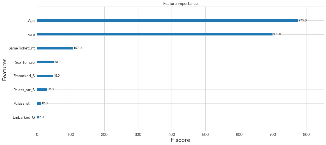
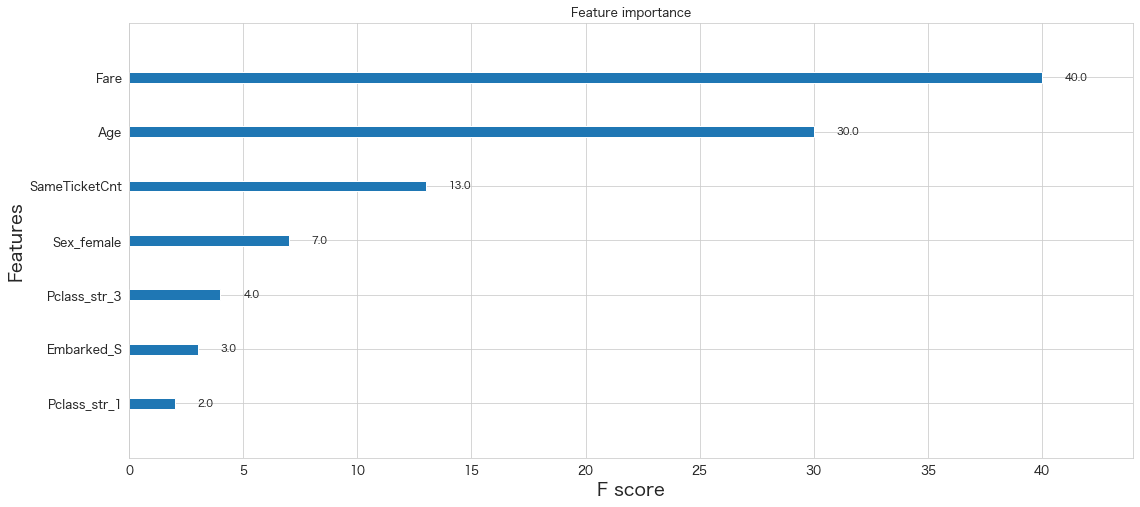
xgb.plot_importance(clf)<AxesSubplot:title={'center':'Feature importance'}, xlabel='F score', ylabel='Features'>
# https://scikit-learn.org/stable/modules/generated/sklearn.metrics.ConfusionMatrixDisplay.html
import matplotlib.pyplot as plt
from sklearn.datasets import make_classification
from sklearn.metrics import ConfusionMatrixDisplay
from sklearn.metrics import confusion_matrix
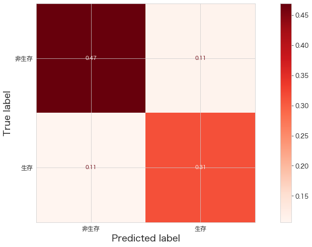
print(confusion_matrix(Y_test,clf.predict(X_test)))
ConfusionMatrixDisplay.from_estimator(clf,X_test,Y_test,cmap="Reds",display_labels=["非生存","生存"],normalize="all")
plt.show()[[84 20]
[19 56]]
Kaggleへ予測データをアップロード
df_eval["Survived"] = clf.predict(df_eval[FEATURE_COLS])
df_eval[["PassengerId","Survived"]].to_csv("titanic_submission.csv",index=False)
!/Users/hinomaruc/Desktop/notebooks/my-venv/bin/kaggle competitions submit -c titanic -f titanic_submission.csv -m "model #008. xgboost"
    100%|████████████████████████████████████████| 2.77k/2.77k [00:05<00:00, 555B/s]
    Successfully submitted to Titanic - Machine Learning from Disaster
0.74880
RandomForestよりはいいけど、、という感じですね。
デフォルトの設定ではなく、GridSearchでパラメーターをチューニングしてみようと思います。
XGBoost (GridSearchでチューニング)
# https://xgboost.readthedocs.io/en/stable/parameter.html
# https://xgboost.readthedocs.io/en/stable/python/python_api.html?#xgboost.XGBClassifier
import xgboost as xgb
from sklearn.metrics import mean_absolute_error
from sklearn.model_selection import GridSearchCV
from sklearn.model_selection import KFold
# Grid Search用のパラメータ作成。
# あまり組み合わせが多いと時間がかかる
params = {
        'eta': [0.1,0.3,0.6],             # default = 0.3
        'gamma': [0,1,2],            # default = 0
        'max_depth': [2,4,6],      # default = 6
        'min_child_weight': [0,1,2],   # default = 1
        'subsample': [0.8,0.9,1],        # default = 1
        'colsample_bytree': [0,0.5,1], # default = 1
        }
# K-分割交差検証
kf = KFold(n_splits = 5, shuffle = True, random_state = 1)
# モデル定義
clf = xgb.XGBClassifier(random_state=10,verbosity=1,use_label_encoder=False)
# Gridサーチ定義
# https://scikit-learn.org/stable/modules/model_evaluation.html#common-cases-predefined-values
grid = GridSearchCV(estimator=clf, param_grid=params, scoring='balanced_accuracy', n_jobs=2, cv=kf.split(X_train,Y_train), verbose=1)scoringは色々な指標があるようです。今回はbalanced_accuracyを選択してみました。各指標についてはもう少し勉強して記事にまとめようと思います。
モデル作成
# fitで学習させる
grid.fit(X_train,Y_train)Fitting 5 folds for each of 729 candidates, totalling 3645 fits in XGBoost 1.3.0, the default evaluation metric used with the objective 'binary:logistic' was changed from 'error' to 'logloss'. Explicitly set eval_metric if you'd like to restore the old behavior. ・・・省略・・・ GridSearchCV(cv=, estimator=XGBClassifier(base_score=None, booster=None, colsample_bylevel=None, colsample_bynode=None, colsample_bytree=None, enable_categorical=False, gamma=None, gpu_id=None, importance_type=None, interaction_constraints=None, learning_rate=None, max_delta_step=None, max_depth=None, min_child_weigh... random_state=10, reg_alpha=None, reg_lambda=None, scale_pos_weight=None, subsample=None, tree_method=None, use_label_encoder=False, validate_parameters=None, verbosity=1), n_jobs=2, param_grid={'colsample_bytree': [0, 0.5, 1], 'eta': [0.1, 0.3, 0.6], 'gamma': [0, 1, 2], 'max_depth': [2, 4, 6], 'min_child_weight': [0, 1, 2], 'subsample': [0.8, 0.9, 1]}, scoring='balanced_accuracy', verbose=1)
# 学習結果確認
print('ベストスコア:',grid.best_score_, sep="\n")
print('\n')
print('ベストestimator:',grid.best_estimator_,sep="\n")
print('\n')
print('ベストparams:',grid.best_params_,sep="\n")
    ベストスコア:
    0.810071880374643

    ベストestimator:
    XGBClassifier(base_score=0.5, booster='gbtree', colsample_bylevel=1,
                  colsample_bynode=1, colsample_bytree=0.5,
                  enable_categorical=False, eta=0.6, gamma=1, gpu_id=-1,
                  importance_type=None, interaction_constraints='',
                  learning_rate=0.600000024, max_delta_step=0, max_depth=2,
                  min_child_weight=1, missing=nan, monotone_constraints='()',
                  n_estimators=100, n_jobs=1, num_parallel_tree=1, predictor='auto',
                  random_state=10, reg_alpha=0, reg_lambda=1, scale_pos_weight=1,
                  subsample=1, tree_method='exact', use_label_encoder=False,
                  validate_parameters=1, verbosity=1)

    ベストparams:
    {'colsample_bytree': 0.5, 'eta': 0.6, 'gamma': 1, 'max_depth': 2, 'min_child_weight': 1, 'subsample': 1}
精度確認
# Grid Searchで一番精度が良かったモデル
best_clf = grid.best_estimator_
# Return the mean accuracy on the given data and labels.
print("train",best_clf.score(X_train,Y_train))
print("test",best_clf.score(X_test,Y_test))
    train 0.8735955056179775
    test 0.8435754189944135
過学習は抑えられたようです。
# モデルパラメータ一覧
best_clf.get_params()
    {'objective': 'binary:logistic',
     'use_label_encoder': False,
     'base_score': 0.5,
     'booster': 'gbtree',
     'colsample_bylevel': 1,
     'colsample_bynode': 1,
     'colsample_bytree': 0.5,
     'enable_categorical': False,
     'gamma': 1,
     'gpu_id': -1,
     'importance_type': None,
     'interaction_constraints': '',
     'learning_rate': 0.600000024,
     'max_delta_step': 0,
     'max_depth': 2,
     'min_child_weight': 1,
     'missing': nan,
     'monotone_constraints': '()',
     'n_estimators': 100,
     'n_jobs': 1,
     'num_parallel_tree': 1,
     'predictor': 'auto',
     'random_state': 10,
     'reg_alpha': 0,
     'reg_lambda': 1,
     'scale_pos_weight': 1,
     'subsample': 1,
     'tree_method': 'exact',
     'validate_parameters': 1,
     'verbosity': 1,
     'eta': 0.6}
xgb.plot_importance(best_clf)<AxesSubplot:title={'center':'Feature importance'}, xlabel='F score', ylabel='Features'>
# https://scikit-learn.org/stable/modules/generated/sklearn.metrics.ConfusionMatrixDisplay.html
import matplotlib.pyplot as plt
from sklearn.datasets import make_classification
from sklearn.metrics import ConfusionMatrixDisplay
from sklearn.metrics import confusion_matrix

print(confusion_matrix(Y_test,best_clf.predict(X_test)))

ConfusionMatrixDisplay.from_estimator(best_clf,X_test,Y_test,cmap="Reds",display_labels=["非生存","生存"],normalize="all")
plt.show()[[96 8]
[20 55]]
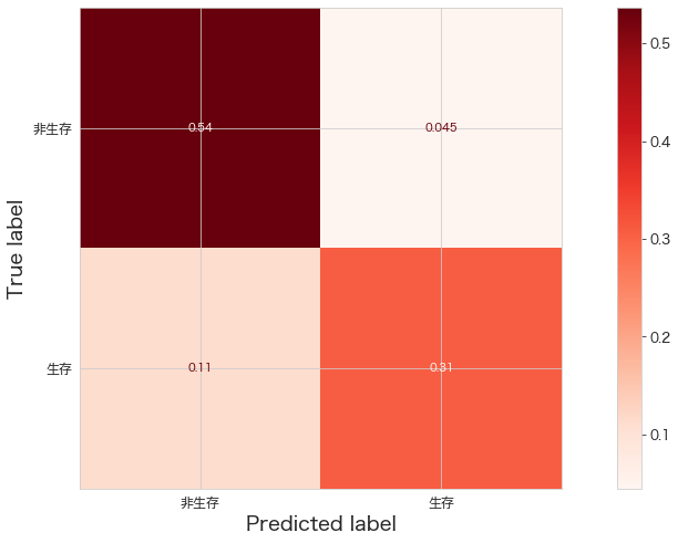
ロジスティック回帰CVの結果は下記なので、それよりはいい結果になっているようです。
[[95 9]
[27 48]]
あとは、実際にKaggleにアップしたときの精度がどうなっているか確認してみます。
Kaggleへ予測データをアップロード
df_eval["Survived"] = best_clf.predict(df_eval[FEATURE_COLS])
df_eval[["PassengerId","Survived"]].to_csv("titanic_submission.csv",index=False)
!/Users/hinomaruc/Desktop/notebooks/my-venv/bin/kaggle competitions submit -c titanic -f titanic_submission.csv -m "model #008. xgboost grid search"
    100%|████████████████████████████████████████| 2.77k/2.77k [00:04<00:00, 578B/s]
    Successfully submitted to Titanic - Machine Learning from Disaster
0.76076
GridSearchを使わない場合より、精度が向上しました。
ただ、ロジスティック回帰CVの精度は0.76794だったので暫定1位の座は奪えませんでした。
まとめ
XGBoostだと0.8は超えるかなと思っていたので、今回作ったモデリング用データだとここら辺の数値が限界なのかもしれません。(それともまだ過学習気味なのか? 訓練データの学習ではテストデータでは表現できていない人物がいるのかもしれません。)
もうちょっと特徴量エンジニアリングを頑張ってみるなど検討の余地はありそうです。
次回はautomlを試してみようと思います。