今回はサポートベクター回帰(SVR)になります。
サポートベクターマシーン(SVM)はよく聞きますが、SVRはSVMを回帰問題に適用したものであるようです。
詳細は「Unlocking the True Power of Support Vector Regression」の記事が分かりやすかったです。
sklearnのSVRは丁寧にも下記の説明をしてくれています。学習の複雑さが増すためデータが1万件以内の場合はSVRを使い、それ以上のデータポイントがある場合は LinearSVRかSGDRegressorをNystoem変換後に利用することを推奨してくれています。
The implementation is based on libsvm. The fit time complexity is more than quadratic with the number of samples which makes it hard to scale to datasets with more than a couple of 10000 samples. For large datasets consider using LinearSVR or SGDRegressor instead, possibly after a Nystroem transformer.引用: https://scikit-learn.org/stable/modules/generated/sklearn.svm.SVR.html
エイムズのデータセットは1万件もないので、SVRを使いたいと思います。
せっかくなのでデフォルトの設定とグリッドサーチでパラメーターを探索する方法の両方を試してみようと思います。
評価指標
住宅IdごとのSalePrice(販売価格)を予測するコンペです。
評価指標は予測SalePriceと実測SalePriceの対数を取ったRoot-Mean-Squared-Error(RMSE)の値のようです。

サポートベクター回帰分析
分析用データの準備
事前に欠損値処理や特徴量エンジニアリングを実施してデータをエクスポートしています。
本記事と同じ結果にするためには事前に下記記事を確認してデータを用意してください。
(その3-2) エイムズの住宅価格のデータセットのデータ加工①
(その3-3) エイムズの住宅価格のデータセットのデータ加工②
学習用データとスコア付与用データの読み込み
import pandas as pd
import numpy as np
# エイムズの住宅価格のデータセットの訓練データとテストデータを読み込む
df = pd.read_csv("/Users/hinomaruc/Desktop/blog/dataset/ames/ames_train.csv")
df_test = pd.read_csv("/Users/hinomaruc/Desktop/blog/dataset/ames/ames_test.csv")
df.head()
Id LotFrontage LotArea LotShape Utilities LandSlope OverallQual OverallCond MasVnrArea ExterCond ... SaleType_New SaleType_Oth SaleType_WD SaleCondition_Abnorml SaleCondition_AdjLand SaleCondition_Alloca SaleCondition_Family SaleCondition_Normal SaleCondition_Partial SalePrice 0 1 65.0 8450 3.0 3.0 2.0 7 5 196.0 2.0 ... 0.0 0.0 1.0 0.0 0.0 0.0 0.0 1.0 0.0 208500 1 2 80.0 9600 3.0 3.0 2.0 6 8 0.0 2.0 ... 0.0 0.0 1.0 0.0 0.0 0.0 0.0 1.0 0.0 181500 2 3 68.0 11250 2.0 3.0 2.0 7 5 162.0 2.0 ... 0.0 0.0 1.0 0.0 0.0 0.0 0.0 1.0 0.0 223500 3 4 60.0 9550 2.0 3.0 2.0 7 5 0.0 2.0 ... 0.0 0.0 1.0 1.0 0.0 0.0 0.0 0.0 0.0 140000 4 5 84.0 14260 2.0 3.0 2.0 8 5 350.0 2.0 ... 0.0 0.0 1.0 0.0 0.0 0.0 0.0 1.0 0.0 250000 5 rows × 335 columns
# 描画設定
from IPython.display import HTML
import seaborn as sns
from matplotlib import ticker
import matplotlib.pyplot as plt
sns.set_style("whitegrid")
from matplotlib import rcParams
rcParams['font.family'] = 'Hiragino Sans' # Macの場合
#rcParams['font.family'] = 'Meiryo' # Windowsの場合
#rcParams['font.family'] = 'VL PGothic' # Linuxの場合
rcParams['xtick.labelsize'] = 12       # x軸のラベルのフォントサイズ
rcParams['ytick.labelsize'] = 12       # y軸のラベルのフォントサイズ
rcParams['axes.labelsize'] = 18        # ラベルのフォントとサイズ
rcParams['figure.figsize'] = 18,8      # 画像サイズの変更(inch)
サポートベクター回帰に使用する変数を選ぶ
重回帰のときと同じにします。
サポートベクター回帰で学習を実施 (デフォルト設定)
# 説明変数と目的変数を指定

# 説明変数
ana_cols=[
  'TotalLivArea'
, 'OverallQual'
, 'TotalBathRms'
, 'GarageCars'
, 'BsmtQual'
, 'FullBath'
, 'GarageFinish'
, 'FireplaceQu'
, 'TotRmsAbvGrd'
#, 'Neighborhood_Blmngtn' avoid multi-correlation
, 'Neighborhood_Blueste'
, 'Neighborhood_BrDale'
, 'Neighborhood_BrkSide'
, 'Neighborhood_ClearCr'
, 'Neighborhood_CollgCr'
, 'Neighborhood_Crawfor'
, 'Neighborhood_Edwards'
, 'Neighborhood_Gilbert'
, 'Neighborhood_IDOTRR'
, 'Neighborhood_MeadowV'
, 'Neighborhood_Mitchel'
, 'Neighborhood_NAmes'
, 'Neighborhood_NPkVill'
, 'Neighborhood_NWAmes'
, 'Neighborhood_NoRidge'
, 'Neighborhood_NridgHt'
, 'Neighborhood_OldTown'
, 'Neighborhood_SWISU'
, 'Neighborhood_Sawyer'
, 'Neighborhood_SawyerW'
, 'Neighborhood_Somerst'
, 'Neighborhood_StoneBr'
, 'Neighborhood_Timber'
, 'Neighborhood_Veenker'
]

# 学習データ
X_train = df[ana_cols]
Y_train = df["SalePrice"] # 販売価格

# テストデータ
X_test = df_test[ana_cols]
# pipelineでデータを標準化してモデリングをする
from sklearn.pipeline import make_pipeline
from sklearn.preprocessing import StandardScaler
# https://scikit-learn.org/stable/modules/generated/sklearn.svm.SVR.html
from sklearn.svm import SVR
pipeline = make_pipeline(StandardScaler(), SVR())
# fitする
fit_pipeline = pipeline.fit(X_train,Y_train)/Users/hinomaruc/Desktop/blog/my-venv/lib/python3.8/site-packages/sklearn/neural_network/_multilayer_perceptron.py:702: ConvergenceWarning: Stochastic Optimizer: Maximum iterations (10000) reached and the optimization hasn't converged yet. warnings.warn(
特にエラーは出ませんでした。
# モデルパラメータ一覧
fit_pipeline.get_params()
    {'memory': None,
     'steps': [('standardscaler', StandardScaler()), ('svr', SVR())],
     'verbose': False,
     'standardscaler': StandardScaler(),
     'svr': SVR(),
     'standardscaler__copy': True,
     'standardscaler__with_mean': True,
     'standardscaler__with_std': True,
     'svr__C': 1.0,
     'svr__cache_size': 200,
     'svr__coef0': 0.0,
     'svr__degree': 3,
     'svr__epsilon': 0.1,
     'svr__gamma': 'scale',
     'svr__kernel': 'rbf',
     'svr__max_iter': -1,
     'svr__shrinking': True,
     'svr__tol': 0.001,
     'svr__verbose': False}
# stepsからニューラルネットワークモデルの部分を抽出
model_pipeline = fit_pipeline.named_steps["svr"] # or pipeline.steps[1][1]
# モデル部分のパラメーターを確認。
model_pipeline.get_params()
    {'C': 1.0,
     'cache_size': 200,
     'coef0': 0.0,
     'degree': 3,
     'epsilon': 0.1,
     'gamma': 'scale',
     'kernel': 'rbf',
     'max_iter': -1,
     'shrinking': True,
     'tol': 0.001,
     'verbose': False}
### モデルを適用し、SalePriceの予測をする
df_test["SalePrice"] = fit_pipeline.predict(X_test)
df_test[["Id","SalePrice"]]
Id SalePrice 0 1461 162903.482999 1 1462 162939.465332 2 1463 163127.384180 3 1464 163133.268749 4 1465 163081.696050 ... ... ... 1454 2915 163038.768807 1455 2916 163038.604298 1456 2917 163027.458012 1457 2918 163003.771370 1458 2919 163104.042927 1459 rows × 2 columns
予測できていそうです。
Kaggleにスコア付与結果をアップロード
df_test[["Id","SalePrice"]].to_csv("ames_submission.csv",index=False)!/Users/hinomaruc/Desktop/blog/my-venv/bin/kaggle competitions submit -c house-prices-advanced-regression-techniques -f ames_submission.csv -m "#5 svr normal"100%|██████████████████████████████████████| 33.8k/33.8k [00:03<00:00, 8.90kB/s] Successfully submitted to House Prices - Advanced Regression Techniques #5 svr normal Score: 0.41621
精度は良くないですね。説明変数が多すぎるのでしょうか? 多項式回帰のときのようにNeighborhood系のダミー変数は除いてもいいのかも知れません。
サポートベクター回帰で学習を実施 (GridSearch利用)
# 説明変数と目的変数を指定

# 説明変数
ana_cols=[
  'TotalLivArea'
, 'OverallQual'
, 'TotalBathRms'
, 'GarageCars'
, 'BsmtQual'
, 'FullBath'
, 'GarageFinish'
, 'FireplaceQu'
, 'TotRmsAbvGrd'
#, 'Neighborhood_Blmngtn' avoid multi-correlation
, 'Neighborhood_Blueste'
, 'Neighborhood_BrDale'
, 'Neighborhood_BrkSide'
, 'Neighborhood_ClearCr'
, 'Neighborhood_CollgCr'
, 'Neighborhood_Crawfor'
, 'Neighborhood_Edwards'
, 'Neighborhood_Gilbert'
, 'Neighborhood_IDOTRR'
, 'Neighborhood_MeadowV'
, 'Neighborhood_Mitchel'
, 'Neighborhood_NAmes'
, 'Neighborhood_NPkVill'
, 'Neighborhood_NWAmes'
, 'Neighborhood_NoRidge'
, 'Neighborhood_NridgHt'
, 'Neighborhood_OldTown'
, 'Neighborhood_SWISU'
, 'Neighborhood_Sawyer'
, 'Neighborhood_SawyerW'
, 'Neighborhood_Somerst'
, 'Neighborhood_StoneBr'
, 'Neighborhood_Timber'
, 'Neighborhood_Veenker'
]

# 学習データ
X_train = df[ana_cols]
Y_train = df["SalePrice"] # 販売価格

# テストデータ
X_test = df_test[ana_cols]
# pipelineでデータを標準化してモデリングをする
from sklearn.pipeline import Pipeline
from sklearn.preprocessing import StandardScaler
from sklearn.model_selection import GridSearchCV
from sklearn.metrics import mean_squared_log_error
# https://scikit-learn.org/stable/modules/generated/sklearn.svm.SVR.html
from sklearn.svm import SVR
# make_pipelineでもOK
pipeline = Pipeline([('scaler', StandardScaler()), ('svr', SVR())])
# グリッドサーチで探索するパラメータ
# 前の行でつけた名前 + __ + 調整したいパラメータ名 で指定できる
param_grid = {
"svr__kernel": ['poly','rbf','sigmoid'], # default: rbf
"svr__degree": [2,3,5], # default: 3
"svr__coef0": [0.0,0.1,0.2], # default:0.0
"svr__tol": [1e-3,1e-2,1e-1], # default:1e-3
"svr__C": [0.5,1.0,1.5], # default:1
"svr__epsilon": [0.1,0.2,0.3] # default:0.1
}
# コンペの評価指標に合わせて、scoringはmean_squared_log_errorにした。
# CVはデフォルトでも5だが、分かりやすいように明示的に指定した。
search = GridSearchCV(pipeline, param_grid, n_jobs=2, scoring='neg_mean_squared_log_error',cv=5,verbose=2)
search.fit(X_train, Y_train)
print("Best parameter (CV score=%0.3f):" % search.best_score_)
print(search.best_params_)
Fitting 5 folds for each of 729 candidates, totalling 3645 fits
[CV] END svr__C=0.5, svr__coef0=0.0, svr__degree=2, svr__epsilon=0.1, svr__kernel=poly, svr__tol=0.001; total time=   0.2s
[CV] END svr__C=0.5, svr__coef0=0.0, svr__degree=2, svr__epsilon=0.1, svr__kernel=poly, svr__tol=0.001; total time=   0.1s
・・・省略・・・
Best parameter (CV score=-0.157):
{'svr__C': 1.5, 'svr__coef0': 0.2, 'svr__degree': 5, 'svr__epsilon': 0.1, 'svr__kernel': 'poly', 'svr__tol': 0.1}
{'svrC': 1.5, 'svrcoef0': 0.2, 'svrdegree': 5, 'svrepsilon': 0.1, 'svrkernel': 'poly', 'svrtol': 0.1}
という結果になりました。
こちらのモデルを利用したいと思います。
# 一番精度が良かったモデル
search.best_estimator_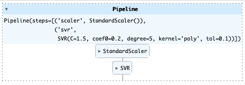
# モデルの適用
best_pipeline_svr = search.best_estimator_
df_test["SalePrice"] = best_pipeline_svr.predict(df_test[ana_cols])

# コンペ提出データの作成
df_test[["Id","SalePrice"]].to_csv("ames_submission.csv",index=False)

# コンペ提出
!/Users/hinomaruc/Desktop/blog/my-venv/bin/kaggle competitions submit -c house-prices-advanced-regression-techniques -f ames_submission.csv -m "#5 svr gridsearch"100%|██████████████████████████████████████| 33.7k/33.7k [00:04<00:00, 7.85kB/s] Successfully submitted to House Prices - Advanced Regression Techniques #5 svr gridsearch 0.41275
むむむ上手く学習できていないようです。
悔しいので、多項式回帰で利用した説明変数で試してみます。
サポートベクター回帰で学習を実施 (GridSearch利用 変数減らす)
# 説明変数と目的変数を指定

# 説明変数
ana_cols=[
  'TotalLivArea'
, 'OverallQual'
, 'TotalBathRms'
, 'GarageCars'
, 'BsmtQual'
, 'FullBath'
, 'GarageFinish'
, 'FireplaceQu'
, 'TotRmsAbvGrd'
]

# 学習データ
X_train = df[ana_cols]
Y_train = df["SalePrice"] # 販売価格

# テストデータ
X_test = df_test[ana_cols]
# pipelineでデータを標準化してモデリングをする
from sklearn.pipeline import Pipeline
from sklearn.preprocessing import StandardScaler
from sklearn.model_selection import GridSearchCV
from sklearn.metrics import mean_squared_log_error
# https://scikit-learn.org/stable/modules/generated/sklearn.svm.SVR.html
from sklearn.svm import SVR
# make_pipelineでもOK
pipeline = Pipeline([('scaler', StandardScaler()), ('svr', SVR())])
# グリッドサーチで探索するパラメータ
# 前の行でつけた名前 + __ + 調整したいパラメータ名 で指定できる
param_grid = {
"svr__kernel": ['poly','rbf','sigmoid'], # default: rbf
"svr__degree": [2,3,5], # default: 3
"svr__coef0": [0.0,0.1,0.2], # default:0.0
"svr__tol": [1e-3,1e-2,1e-1], # default:1e-3
"svr__C": [0.5,1.0,1.5], # default:1
"svr__epsilon": [0.1,0.2,0.3] # default:0.1
}
# コンペの評価指標に合わせて、scoringはmean_squared_log_errorにした。
# CVはデフォルトでも5だが、分かりやすいように明示的に指定した。
search = GridSearchCV(pipeline, param_grid, n_jobs=2, scoring='neg_mean_squared_log_error',cv=5,verbose=2)
search.fit(X_train, Y_train)
print("Best parameter (CV score=%0.3f):" % search.best_score_)
print(search.best_params_)
Fitting 5 folds for each of 729 candidates, totalling 3645 fits
[CV] END svr__C=0.5, svr__coef0=0.0, svr__degree=2, svr__epsilon=0.1, svr__kernel=poly, svr__tol=0.001; total time=   0.2s
・・・省略・・・
[CV] END svr__C=1.5, svr__coef0=0.2, svr__degree=3, svr__epsilon=0.2, svr__kernel=poly, svr__tol=0.1; total time=   0.2s

Best parameter (CV score=-0.144):
{'svr__C': 1.5, 'svr__coef0': 0.2, 'svr__degree': 5, 'svr__epsilon': 0.3, 'svr__kernel': 'poly', 'svr__tol': 0.001}
# 一番精度が良かったモデル
search.best_estimator_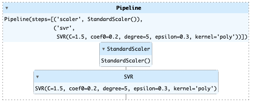
# モデルの適用
best_pipeline_svr = search.best_estimator_
df_test["SalePrice"] = best_pipeline_svr.predict(df_test[ana_cols])

# コンペ提出データの作成
df_test[["Id","SalePrice"]].to_csv("ames_submission.csv",index=False)

# コンペ提出
!/Users/hinomaruc/Desktop/blog/my-venv/bin/kaggle competitions submit -c house-prices-advanced-regression-techniques -f ames_submission.csv -m "#5 svr gridsearch 2"100%|██████████████████████████████████████| 33.7k/33.7k [00:03<00:00, 8.88kB/s] Successfully submitted to House Prices - Advanced Regression Techniques #5 svr gridsearch 2 0.39084
ぐっあまり精度はあがりませんでした。
使用ライブラリのバージョン
pandas Version: 1.4.3
numpy Version: 1.22.4
scikit-learn Version: 1.1.1
seaborn Version: 0.11.2
matplotlib Version: 3.5.2
まとめ
残念ながら精度はかなり悪い結果となってしまいました。
SVRはデータを標準化しちゃいけなかったかな?とも思ったのですが標準化した方がベターなようです。
It is better to have the same scale in many optimization methods.
Many kernel functions use internally an euclidean distance to compare two different samples (in the gaussian kernel the euclidean distance is in the exponential term), if every feature has a different scale, the euclidean distance only take into account the features with highest scale. 引用: https://stackoverflow.com/questions/40531152/is-there-a-need-to-normalise-input-vector-for-prediction-in-svm
後はscoringがよくなかったかなー色々試してみたいところですがここまでにしておきます。
次回はRandom Foresetを試してみます。
参考
・https://scikit-learn.org/stable/tutorial/statistical_inference/putting_together.html