MaskRCNNによる物体検知を試してみるの記事の続きになります。
前回はdetectメソッドで物体検知を試しました。今回はAPの計算をしてみようと思います。
サンプルを確認するとutilsのcompute_apメソッドで実現可能そうです。
Draw precision-recall curve
AP, precisions, recalls, overlaps = utils.compute_ap(gt_bbox, gt_class_id, gt_mask,
r['rois'], r['class_ids'], r['scores'], r['masks'])
visualize.plot_precision_recall(AP, precisions, recalls)
引用: https://github.com/matterport/Mask_RCNN/blob/master/samples/coco/inspect_model.ipynb
ground truthはbboxとmask両方の値をcompute_apの引数として投入しているようですが、IoUはmaskを使っている様です。
overlaps = compute_overlaps_masks(pred_masks, gt_masks)
引用: https://github.com/matterport/Mask_RCNN/blob/master/mrcnn/utils.py#LL681C1-L682C60
また、compute_ap_rangeメソッドではcoco metricみたいにIoUが0.5から0.95の間0.05刻みでAPを計算し平均値を計算してくれるようです。
def compute_ap_range(gt_box, gt_class_id, gt_mask,
pred_box, pred_class_id, pred_score, pred_mask,
iou_thresholds=None, verbose=1):
"""Compute AP over a range or IoU thresholds. Default range is 0.5-0.95."""
Default is 0.5 to 0.95 with increments of 0.05
引用: https://github.com/matterport/Mask_RCNN/blob/master/mrcnn/utils.py#L754
精度を計算するには兎にも角にも正解データが必要なので、YOLOv8のときと同じ様にアノテーションを作成します。
インスタンスセグメンテーションなので車の形を正確にポリゴン(マスク)としてデータ化します。これは次のセクションでやってみます。
余談ですが、YOLOv8でもセグメンテーションタスクは実行できます。詳細は公式ページ「Segment」の項目にて確認できます。COCOフォーマットからYOLOフォーマットに変換する処理もYOLOv8では用意されているようです。
from ultralytics.yolo.data.converter import convert_coco
convert_coco(labels_dir='../coco/annotations/', use_segments=True)
引用: https://docs.ultralytics.com/datasets/segment/
利用する画像データは1枚だけだと実用性に欠けるので2枚利用することにしました。(640pxにリサイズしました)
Ground Truthの作成 (インスタンス・セグメンテーション)
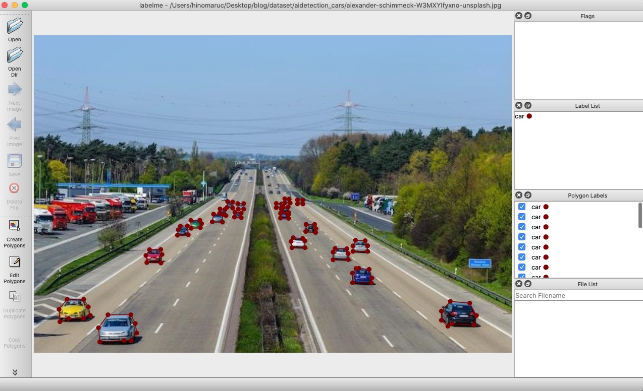
世の中には色々なアノテーションツールがありますが、今回はlabelmeというツールを使いました。
公式サンプルのballoon.pyを参考に独自データセットですぐMask R-CNNで学習をしたいという方はVGG Image Annotatorというツールを使うと良いと思います。アノテーションした出力結果をそのまま読み込むことが出来ます。
labelmeはlabelmeのjsonフォーマットからVOCフォーマットやCOCOフォーマットに出力可能なようです。
Exporting VOC-format dataset for semantic/instance segmentation. (semantic segmentation, instance segmentation)
Exporting COCO-format dataset for instance segmentation. (instance segmentation)
引用: https://github.com/wkentaro/labelme
変換方法はサンプルがありますので参考にしつつ実行してみます。labelme2voc.pyやlabelme2coco.pyというスクリプトが用意されているので実行するだけで良い様です。
{
  "version": "5.2.1",
  "flags": {},
  "shapes": [
    {
      "label": "car",
      "points": [
        [
          473.0405405405406,
          351.4864864864865
        ],
        [
          433.17567567567573,
          352.83783783783787
        ],
        [
          415.6081081081081,
          356.89189189189193
        ],
        [
          412.22972972972974,
          369.05405405405406
        ],
        [
          414.2567567567568,
          387.97297297297297
        ],
        [
          435.20270270270277,
          419.05405405405406
        ],
        [
          441.2837837837838,
          425.13513513513516
        ],
        [
          503.445945945946,
          421.0810810810811
        ],
        [
          506.1486486486487,
          396.0810810810811
        ]
      ],
      "group_id": null,
      "description": "",
      "shape_type": "polygon",
      "flags": {}
    }
  ],
  "imagePath": "maksim-tarasov-bFTVxTo266E-unsplash.jpg",
  "imageData": "省略",
  "imageHeight": 480,
  "imageWidth": 640
}
今回はよく使うCOCOフォーマットに変換してみます。
labelmeのプロジェクトをcloneした後、下記のようにlabelmeでアノテーションした画像とjsonファイルをdata_annotatedフォルダに配置、data_dataset_cocoフォルダを削除、labels.txtに記載するクラスをCOCOのモデルに使っているクラスに変更しています。
labels.txtの先頭行「ignore」はないとエラーになったのでサンプルのままにしてあります。エラーは「issue with running labelme2coco #852」に記載されている通りでした。また、「background」は無くても変換時にエラーにはなりませんでしたが、MatterportのMask R-CNNでDatasetクラスのインスタンスを作った際にError: Class id for "person" cannot be less than one. (0 is reserved for the background)になったので_background_を変換時に利用し、後から削除することによってクラスIDを1から採番するようにした方が良さそうです。
(venv-maskrcnn) git clone https://github.com/wkentaro/labelme.git
(venv-maskrcnn) pwd
/Users/hinomaruc/Desktop/blog/labelme/examples/instance_segmentation
(venv-maskrcnn) ls data_annotated
alexander-schimmeck-W3MXYIfyxno-unsplash.jpg
alexander-schimmeck-W3MXYIfyxno-unsplash.json
maksim-tarasov-bFTVxTo266E-unsplash.jpg
maksim-tarasov-bFTVxTo266E-unsplash.json
(venv-maskrcnn) rm -rf data_dataset_coco
(venv-maskrcnn) cat labels.txt
__ignore__
_background_
person
bicycle
car
motorcycle
airplane
bus
train
truck
boat
traffic light
fire hydrant
stop sign
parking meter
bench
bird
cat
dog
horse
sheep
cow
elephant
bear
zebra
giraffe
backpack
umbrella
handbag
tie
suitcase
frisbee
skis
snowboard
sports ball
kite
baseball bat
baseball glove
skateboard
surfboard
tennis racket
bottle
wine glass
cup
fork
knife
spoon
bowl
banana
apple
sandwich
orange
broccoli
carrot
hot dog
pizza
donut
cake
chair
couch
potted plant
bed
dining table
toilet
tv
laptop
mouse
remote
keyboard
cell phone
microwave
oven
toaster
sink
refrigerator
book
clock
vase
scissors
teddy bear
hair drier
toothbrush./labelme2coco.py data_annotated data_dataset_coco --labels labels.txtCreating dataset: data_dataset_coco Generating dataset from: data_annotated/alexander-schimmeck-W3MXYIfyxno-unsplash.json Generating dataset from: data_annotated/maksim-tarasov-bFTVxTo266E-unsplash.json
{"images": [
    {"license": 0, "url": null, "file_name": "JPEGImages/alexander-schimmeck-W3MXYIfyxno-unsplash.jpg", "height": 426, "width": 640, "date_captured": null, "id": 0},
    {"license": 0, "url": null, "file_name": "JPEGImages/maksim-tarasov-bFTVxTo266E-unsplash.jpg", "height": 480, "width": 640, "date_captured": null, "id": 1}],

"annotations": [
    {"id": 0, "image_id": 0, "category_id": 3, "segmentation": [[44.662162162162176, 354.21621621621625, 66.95945945945948, 354.21621621621625, 73.04054054054056, 364.35135135135135, 75.74324324324327, 375.83783783783787, 66.2837837837838, 379.89189189189193, 46.666666666666664, 380.0, 35.0, 384.3333333333333, 33.85135135135136, 367.72972972972974]], "area": 971.0, "bbox": [33.0, 354.0, 43.0, 31.0], "iscrowd": 0},
    {"id": 1, "image_id": 0, "category_id": 3, "segmentation": [[155.0, 287.6666666666667, 150.06756756756758, 295.43243243243245, 151.33333333333334, 305.0, 170.33783783783784, 305.5675675675676, 171.6891891891892, 294.0810810810811, 170.0, 287.3333333333333]], "area": 379.0, "bbox": [150.0, 287.0, 22.0, 19.0], "iscrowd": 0}, {"id": 2, "image_id": 0, "category_id": 3, "segmentation": [[99.33333333333333, 375.0, 86.66666666666667, 392.3333333333333, 88.33333333333333, 411.3333333333333, 121.01351351351353, 409.6216216216216, 130.47297297297297, 409.6216216216216, 137.90540540540542, 399.4864864864865, 135.8783783783784, 386.64864864864865, 130.0, 375.0]], "area": 1600.0, "bbox": [86.0, 375.0, 52.0, 37.0], "iscrowd": 0},...省略...],

"categories": [{"supercategory": null, "id": 0, "name": "_background_"}, {"supercategory": null, "id": 1, "name": "person"}, {"supercategory": null, "id": 2, "name": "bicycle"}, {"supercategory": null, "id": 3, "name": "car"}...省略...]
}
COCOフォーマットで出力出来ている様です。
精度を確認するのに必要なクラスの定義などの情報一覧
精度を確認するのに最終的に実行したいのはutils.compute_apメソッドですが、引数としてgt_bbox, gt_class_id, gt_mask, r['rois'], r['class_ids'], r['scores'], r['masks']が必要になります。
r['rois'], r['class_ids'], r['scores'], r['masks']はdetectした結果から取得できるのでシンプルですね。
gt_bbox, gt_class_id, gt_maskはmrcnn/model.pyのload_image_gtメソッドの返却値から取得することが出来ます。bboxやmaskの値だけであればアノテーションファイルからもパースすることで取得可能ですが、compute_apメソッド内の処理で画像のリサイズなども行われる様で素直に用意されている処理を活用することにしました。
load_image_gtですが、引数としてdataset, config, image_idが求められます。
datasetはMatterportのMask R-CNNで用意されているクラスをインスタンス化したものです。アノテーションファイルなどからimage_idやpolygonデータを取得し保持するために使います。訓練データや検証データを読み込む時に使われています。
Datasetクラスのコードのコメント蘭にはデータセットによって関数を追加するなどし新しいDatasetクラスを作成してくださいと記載されています。今回はCOCOフォーマットのアノテーションを読み込めるDatasetクラスを作成しました。(といってもmask-rcnn-training-with-coco-like-dataset-in-colabを参考にしただけですが 笑)
To use it, create a new class that adds functions specific to the dataset you want to use
引用: https://github.com/matterport/Mask_RCNN/blob/master/mrcnn/utils.py#L239
configはmrcnn.configから定義してもいいですし、サンプルのcoco.pyなどを読み込んで作成するでもOKです。今回はmrcnn.configから定義しようと思います。
image_idは分かっていれば自分で入力するか、datasetオブジェクトから取得することになります。今回はdatasetオブジェクトから取得します。
lablemeで作成したアノテーションファイルの修正
Datasetクラスのインスタンスを作成しデータをロードする時にエラーになるので、事前にアノテーションファイルを修正しておきます。ちなみにこの作業はlableme利用してアノテーションファイルを作成しCOCOフォーマットに変換した もしくは MatterportのMask R-CNNを利用する場合の話で他のアノテーションツールやMask R-CNNのライブラリだと問題なく動く可能性があります。
修正内容は下記:
- "categories": [{"supercategory": null, "id": 0, "name": "background"}を除外
- file_nameからJPEGImages/を除外
import json

coco_anno_dir = "/Users/hinomaruc/Desktop/blog/labelme/examples/instance_segmentation/data_dataset_coco"
annotation_file = os.path.join(coco_anno_dir, 'annotations.json')
modified_file = os.path.join(coco_anno_dir, 'annotations_mod.json')

with open(annotation_file, 'r') as file:
    data = json.load(file)

# 1. "categories": [{"supercategory": null, "id": 0, "name": "_background_"}を除外
data['categories'] = [category for category in data['categories'] if category['id'] != 0]

# 2. file_nameからJPEGImages/を除外
for image in data['images']:
    image['file_name'] = image['file_name'].replace('JPEGImages/', '')

with open(modified_file, 'w') as file:
    json.dump(data, file)
COCOフォーマット読み込み用のDatasetクラスを作成しテスト用データセットオブジェクトを作成する
import os
import sys
import random
import math
import re
import time
import numpy as np
import tensorflow as tf
import matplotlib
import matplotlib.pyplot as plt
import matplotlib.patches as patches
# ルートの設定
ROOT_DIR = os.path.abspath("/Users/hinomaruc/Desktop/blog/Mask_RCNN")
# Mask R-CNN関連のパッケージのインポート
sys.path.append(ROOT_DIR)
from mrcnn import utils
from mrcnn import visualize
from mrcnn.visualize import display_images
import mrcnn.model as modellib
from mrcnn.model import log
from PIL import Image, ImageDraw
# ログディレクトリ
MODEL_DIR = os.path.join(ROOT_DIR, "logs")
# 学習用のモデルweightファイル
COCO_MODEL_PATH = os.path.join(ROOT_DIR, "mask_rcnn_coco.h5")
# CocoFormatDatasetクラスの定義
class CocoFormatDataset(utils.Dataset):
def load_data(self, annotation_json, images_dir):
""" Load the your dataset
annotation_json: The path to the coco annotations json file
images_dir: The directory holding the images referred to by the json file
"""
# アノテーションファイルの読み込み
json_file = open(annotation_json)
coco_json = json.load(json_file)
json_file.close()
# utils.Datasetのadd_classメソッドでクラス名を追加
source_name = "coco"
for category in coco_json['categories']:
class_id = category['id']
class_name = category['name']
if class_id < 1:
print('Error: Class id for "{}" cannot be less than one. (0 is reserved for the background)'.format(
class_name))
return
self.add_class(source_name, class_id, class_name)
# アノテーションの取得
annotations = {}
for annotation in coco_json['annotations']:
image_id = annotation['image_id']
if image_id not in annotations:
annotations[image_id] = []
annotations[image_id].append(annotation)
# 画像情報の取得
seen_images = {}
for image in coco_json['images']:
image_id = image['id']
if image_id in seen_images:
print("Warning: Skipping duplicate image id: {}".format(image))
else:
seen_images[image_id] = image
try:
image_file_name = image['file_name']
image_width = image['width']
image_height = image['height']
except KeyError as key:
print("Warning: Skipping image (id: {}) with missing key: {}".format(image_id, key))
image_path = os.path.abspath(os.path.join(images_dir, image_file_name))
image_annotations = annotations[image_id]
# utils.Datasetのadd_imageメソッドで画像情報を追加
self.add_image(
source=source_name,
image_id=image_id,
path=image_path,
width=image_width,
height=image_height,
annotations=image_annotations
)
def load_mask(self, image_id):
""" Load instance masks for the given image.
MaskRCNN expects masks in the form of a bitmap [height, width, instances].
Args:
image_id: The id of the image to load masks for
Returns:
masks: A bool array of shape [height, width, instance count] with
one mask per instance.
class_ids: a 1D array of class IDs of the instance masks.
"""
image_info = self.image_info[image_id]
annotations = image_info['annotations']
instance_masks = []
class_ids = []
for annotation in annotations:
class_id = annotation['category_id']
mask = Image.new('1', (image_info['width'], image_info['height']))
mask_draw = ImageDraw.ImageDraw(mask, '1')
for segmentation in annotation['segmentation']:
mask_draw.polygon(segmentation, fill=1)
bool_array = np.array(mask) > 0
instance_masks.append(bool_array)
class_ids.append(class_id)
mask = np.dstack(instance_masks)
class_ids = np.array(class_ids, dtype=np.int32)
return mask, class_ids
# テスト用画像とcocoフォーマットのアノテーションの場所
coco_anno_dir="/Users/hinomaruc/Desktop/blog/labelme/examples/instance_segmentation/data_dataset_coco"
coco_anno_json=os.path.join(coco_anno_dir,'annotations_mod.json')
test_images=os.path.join(coco_anno_dir,"JPEGImages")
# データセットの作成
dataset_test = CocoFormatDataset()
dataset_test.load_data(coco_anno_json, test_images)
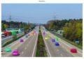
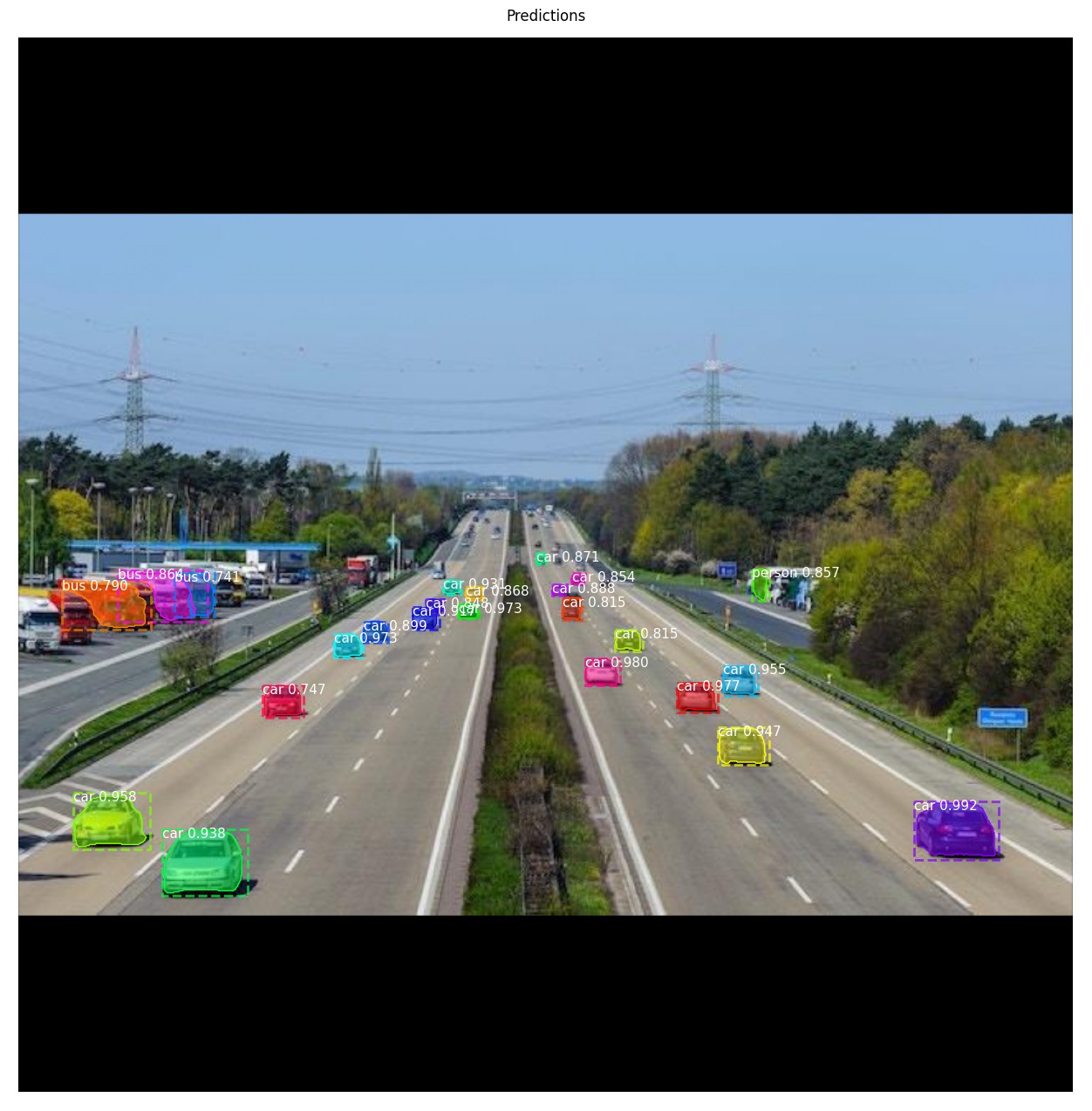
dataset_test.prepare()Mask R-CNNでテスト画像に存在するオブジェクトを検知してみる (1枚目)
今回は2枚のテストデータの精度を確認するので、同じ様なコードが繰り返すことになります。
まずは1枚目の車両がたくさん存在する画像からです。
# 訓練用の設定を定義
from mrcnn.config import Config
class myOwnCocoConfig(Config):
    NAME = "myOwnCocoConfig"
    IMAGES_PER_GPU = 2
    NUM_CLASSES = 1 + 80  # background + 80クラス
config = myOwnCocoConfig()

# 学習用の設定を上書きし推論用のパラメータを設定する
class InferenceConfig(config.__class__):
    GPU_COUNT = 1
    IMAGES_PER_GPU = 1

config = InferenceConfig()

## デバイスとモードの設定
DEVICE = "/cpu:0"  # /cpu:0 or /gpu:0
TEST_MODE = "inference"

# モデルの設定読み込み
with tf.device(DEVICE):
    model = modellib.MaskRCNN(mode="inference", model_dir=MODEL_DIR,config=config)
model.load_weights(COCO_MODEL_PATH, by_name=True)

image_id = dataset_test.image_ids[0]
image, image_meta, gt_class_id, gt_bbox, gt_mask = modellib.load_image_gt(dataset_test, config, image_id, use_mini_mask=False)
info = dataset_test.image_info[image_id]
print("image ID: {}.{} ({}) {}".format(info["source"], info["id"], image_id, dataset_test.image_reference(image_id)))

# 推論の実施
results = model.detect([image], verbose=1)

# 描画用の設定
def get_ax(rows=1, cols=1, size=16):
    """Return a Matplotlib Axes array to be used in
    all visualizations in the notebook. Provide a
    central point to control graph sizes.

    Adjust the size attribute to control how big to render images
    """
    _, ax = plt.subplots(rows, cols, figsize=(size*cols, size*rows))
    return ax

# 推論結果の描画
ax = get_ax(1)
r = results[0]
visualize.display_instances(image, r['rois'], r['masks'], r['class_ids'],
                            dataset_test.class_names, r['scores'], ax=ax,
title="Predictions")image ID: coco.0 (0) Processing 1 images image shape: (1024, 1024, 3) min: 0.00000 max: 255.00000 uint8 molded_images shape: (1, 1024, 1024, 3) min: -123.70000 max: 151.10000 float64 image_metas shape: (1, 93) min: 0.00000 max: 1024.00000 int64 anchors shape: (1, 261888, 4) min: -0.35390 max: 1.29134 float32
Average Precisionで精度を算出 (1枚目)
やっとやりたかったことが出来ますね 笑 utils.compute_apメソッドを実行してみます。
AP, precisions, recalls, overlaps = utils.compute_ap(gt_bbox, gt_class_id, gt_mask,r['rois'], r['class_ids'], r['scores'], r['masks'])
print("AP=",AP)
visualize.plot_precision_recall(AP, precisions, recalls)AP= 0.8221877262644146
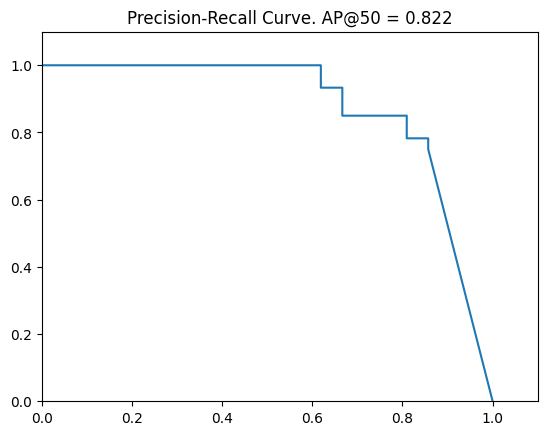
0.822といい精度ではないでしょうか。
Ground Truthとマッチした検知結果との対応表 (1枚目)
visualize.plot_overlaps(gt_class_id, r['class_ids'], r['scores'],overlaps, dataset_test.class_names)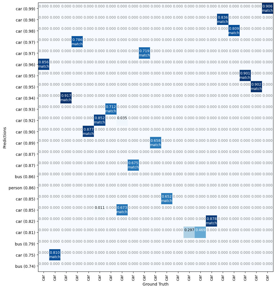
正解データでアノテーションした車両のうち2台はconfidenceが低いのでマッチしていないことが分かりますね。
正解データと検知結果の比較 (1枚目)
正解ラベルと比較することで推論とのズレが確認しやすくなりますね。
visualize.display_differences(
    image,
    gt_bbox, gt_class_id, gt_mask,
    r['rois'], r['class_ids'], r['scores'], r['masks'],
    dataset_test.class_names, ax=get_ax(),
    show_box=False, show_mask=False,
    iou_threshold=0.5, score_threshold=0.5)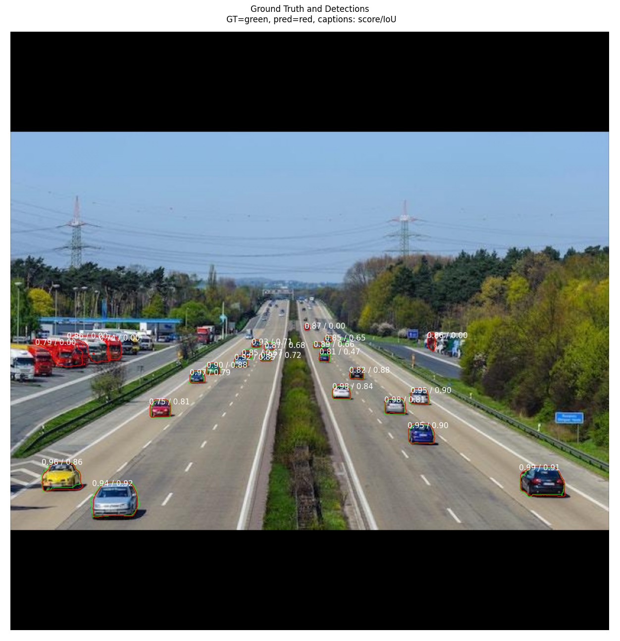
赤が正解ラベルで緑が検知ラベルです。数字はconfidence / IoU値になっているようです。
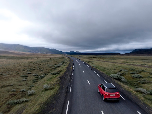
2枚目のテスト画像の物体検知と精度算出
2枚目のテスト画像は車両が1台だけのものを選択しました。確認してみます。
image_id = dataset_test.image_ids[1]

image, image_meta, gt_class_id, gt_bbox, gt_mask = modellib.load_image_gt(dataset_test, config, image_id, use_mini_mask=False)
info = dataset_test.image_info[image_id]
print("image ID: {}.{} ({}) {}".format(info["source"], info["id"], image_id, dataset_test.image_reference(image_id)))

# 推論の実施
results = model.detect([image], verbose=1)

# 推論結果の描画
ax = get_ax(1)
r = results[0]
visualize.display_instances(image, r['rois'], r['masks'], r['class_ids'],
                            dataset_test.class_names, r['scores'], ax=ax,
title="Predictions")image ID: coco.1 (1) Processing 1 images image shape: (1024, 1024, 3) min: 0.00000 max: 255.00000 uint8 molded_images shape: (1, 1024, 1024, 3) min: -123.70000 max: 151.10000 float64 image_metas shape: (1, 93) min: 0.00000 max: 1024.00000 int64 anchors shape: (1, 261888, 4) min: -0.35390 max: 1.29134 float32
きちんと検知出来ている様です。
Average Precisionで精度を確認 (2枚目)
AP, precisions, recalls, overlaps = utils.compute_ap(gt_bbox, gt_class_id, gt_mask,r['rois'], r['class_ids'], r['scores'], r['masks'])
print("AP=",AP)
visualize.plot_precision_recall(AP, precisions, recalls)AP= 1.0
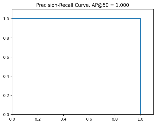
画像に1台しかない車両を検知することが出来たのでAP=1になりました。
Ground Truthとマッチした検知結果との対応表 (2枚目)
visualize.plot_overlaps(gt_class_id, r['class_ids'], r['scores'],overlaps, dataset_test.class_names)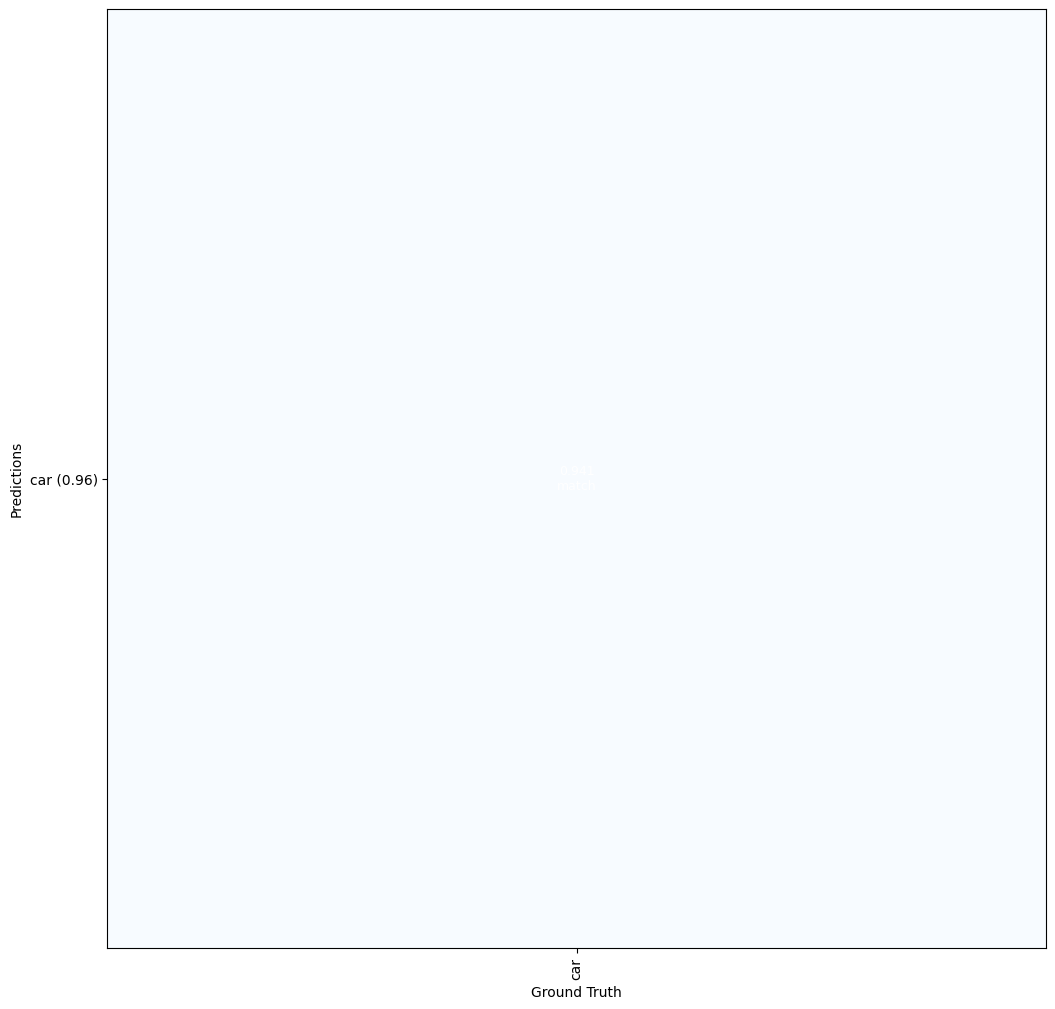
正解データと検知結果の比較 (2枚目)
visualize.display_differences(
    image,
    gt_bbox, gt_class_id, gt_mask,
    r['rois'], r['class_ids'], r['scores'], r['masks'],
    dataset_test.class_names, ax=get_ax(),
    show_box=False, show_mask=False,
    iou_threshold=0.5, score_threshold=0.5)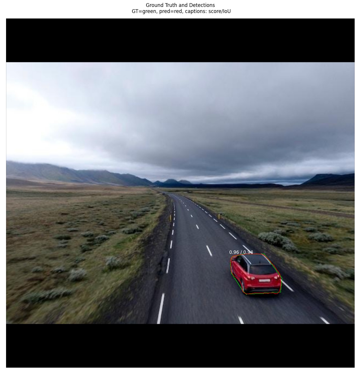
複数枚数のAverage Precisionを計算する方法
実際は複数枚をまとめて精度確認することの方が多いのではないでしょうか。単純にAPの平均を計算するだけで良い様です。
def compute_batch_ap(dataset):
    APs = []
    for image_id in dataset.image_ids:
        image, image_meta, gt_class_id, gt_bbox, gt_mask = modellib.load_image_gt(dataset, config, image_id, use_mini_mask=False)
        results = model.detect([image], verbose=0)
        r = results[0]
        AP, precisions, recalls, overlaps = utils.compute_ap(gt_bbox, gt_class_id, gt_mask, r['rois'], r['class_ids'], r['scores'], r['masks'])
        APs.append(AP)
    return APs

APs = compute_batch_ap(dataset_test)
print("mAP @ IoU=50: ", np.mean(APs))mAP @ IoU=50: 0.9110938631322073
IoUのレンジを変えてAPを計算
COCO metricみたいに0.5から0.95までIoUの閾値を0.05ずつ増やしながらAPを計算する方法です。
テスト画像1枚目
# image_idの指定
image_id = dataset_test.image_ids[0]

# ground truthデータの読み込み
image, image_meta, gt_class_id, gt_bbox, gt_mask = modellib.load_image_gt(dataset_test, config, image_id, use_mini_mask=False)

# 推論の実施
results = model.detect([image], verbose=1)

# 結果の格納
r = results[0]

# APの計算 (IoUは0.5から0.95)
utils.compute_ap_range(gt_bbox, gt_class_id, gt_mask,r['rois'], r['class_ids'], r['scores'], r['masks'],verbose=1)Processing 1 images image shape: (1024, 1024, 3) min: 0.00000 max: 255.00000 uint8 molded_images shape: (1, 1024, 1024, 3) min: -123.70000 max: 151.10000 float64 image_metas shape: (1, 93) min: 0.00000 max: 1024.00000 int64 anchors shape: (1, 261888, 4) min: -0.35390 max: 1.29134 float32 AP @0.50: 0.822 AP @0.55: 0.822 AP @0.60: 0.822 AP @0.65: 0.822 AP @0.70: 0.631 AP @0.75: 0.490 AP @0.80: 0.409 AP @0.85: 0.233 AP @0.90: 0.111 AP @0.95: 0.000 AP @0.50-0.95: 0.516 0.5163768219092078
IoUの閾値が高くなるにつれAPも低くなります。(基準が厳しくなるため)
テスト画像2枚目
# image_idの指定
image_id = dataset_test.image_ids[1]

# ground truthデータの読み込み
image, image_meta, gt_class_id, gt_bbox, gt_mask = modellib.load_image_gt(dataset_test, config, image_id, use_mini_mask=False)

# 推論の実施
results = model.detect([image], verbose=1)

# 結果の格納
r = results[0]

# APの計算 (IoUは0.5から0.95)
utils.compute_ap_range(gt_bbox, gt_class_id, gt_mask,r['rois'], r['class_ids'], r['scores'], r['masks'],verbose=1)Processing 1 images image shape: (1024, 1024, 3) min: 0.00000 max: 255.00000 uint8 molded_images shape: (1, 1024, 1024, 3) min: -123.70000 max: 151.10000 float64 image_metas shape: (1, 93) min: 0.00000 max: 1024.00000 int64 anchors shape: (1, 261888, 4) min: -0.35390 max: 1.29134 float32 AP @0.50: 1.000 AP @0.55: 1.000 AP @0.60: 1.000 AP @0.65: 1.000 AP @0.70: 1.000 AP @0.75: 1.000 AP @0.80: 1.000 AP @0.85: 1.000 AP @0.90: 1.000 AP @0.95: 0.000 AP @0.50-0.95: 0.900 0.9
一見完璧だと思われた2枚目でさえもAP@0.95ではAP=0という結果になります。
まとめ
いかがでしたでしょうか?MatterportのMask R-CNNでは最初から便利なメソッドが用意されているので簡単に精度を確認することが出来ましたね。
他にも作成したモデルの中身を詳しくみるためのメソッドなどが用意されているので、サンプルをみるだけでもMask R-CNNの勉強になります。