物体検知の案件をやっていると物体数をカウントしたい場合が多いかと思います。
この場合、model.detectを実行して検出されたクラスのバウンディングボックスの数をカウントしてあげれば、画像や動画内の物体数をカウントすることが出来ます。
ただ実業務では、画像全体が対象ではなく領域を絞って物体検知や物体数のカウントしたいという要件もあるのではないでしょうか。
本記事では下記ハイウェイの画像を元に、道路を通ってる車の数を左側のレーンや右側のレーンごとなどエリアを区切って検知/カウントしてみようと思います。
※ 検知は画像全体に対して実施しますが、bboxの位置で表示する検知物体や精度を計算する領域を決めてフィルタリングするという方が正しいかも知れません。本当に物体検知を特定の領域のみを対象にしたい場合は「YOLOv8で特定のエリアのみ物体検知する方法」で行ったように黒いマスク画像を用意して、元画像にオーバーラップしてあげることで実現可能です。
画像はunsplash.comからダウンロードしました。ドイツの高速道路のようです。ダウンロード後に640pxになるように縮小しました。
奥の方の車両は小さすぎて検知対象に加えたくはないし、トラックがたくさん駐車している箇所も検知箇所からは除外したいですね。
Ground Truthデータの作成
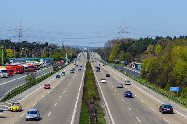
まずはGround Truthデータとして正解データを作成するため、車両をアノテーションしました。全部で21台アノテーションしました。
この作業を丁寧にやらないと精度確認に影響がありますので集中してやります 笑
LableImgでアノテーションしたと仮定しています。下記で描画していますが、LabelImgではxywhnフォーマットのtxtファイルが出力されるので、xyxyフォーマットに変換して描画しています。
ラベルはYOLOv8のpremodelに合わせて、2:carに設定しています。
from PIL import Image, ImageDraw

# 画像の読み込み
image = Image.open("/Users/hinomaruc/Desktop/blog/dataset/aidetection_cars/alexander-schimmeck-W3MXYIfyxno-unsplash.jpg")

# アノテーションしたファイルの読み込み
with open("/Users/hinomaruc/Desktop/blog/dataset/aidetection_cars/alexander-schimmeck-W3MXYIfyxno-unsplash.txt", "r") as file:
    lines = file.readlines()

# 描画オブジェクトの作成
draw = ImageDraw.Draw(image)

# YOLOフォーマットtxtの読み込み
for line in lines:

    line = line.strip().split(" ")

    # LabelImgで作成したので、class + xywhnフォーマットになっている
    class_index = int(line[0]) # クラス番号
    x_normalized = float(line[1]) # 標準化済みx
    y_normalized = float(line[2]) # 標準化済みy
    width_normalized = float(line[3]) # 標準化済みwidth
    height_normalized = float(line[4]) # 標準化済みheight

    # 標準化xywhをピクセル値に変換する
    width, height = image.size # 画像サイズの取得
    x_pixel = int(x_normalized * width)
    y_pixel = int(y_normalized * height)
    width_pixel = int(width_normalized * width)
    height_pixel = int(height_normalized * height)

    # xyxyフォーマットに変換
    x1 = x_pixel - (width_pixel // 2)
    y1 = y_pixel - (height_pixel // 2)
    x2 = x_pixel + (width_pixel // 2)
    y2 = y_pixel + (height_pixel // 2)

    # bboxを描画する
    draw.rectangle([(x1, y1), (x2, y2)], outline="red", width=1)

# 保存
image.save("labeled_image.jpg")
image.show()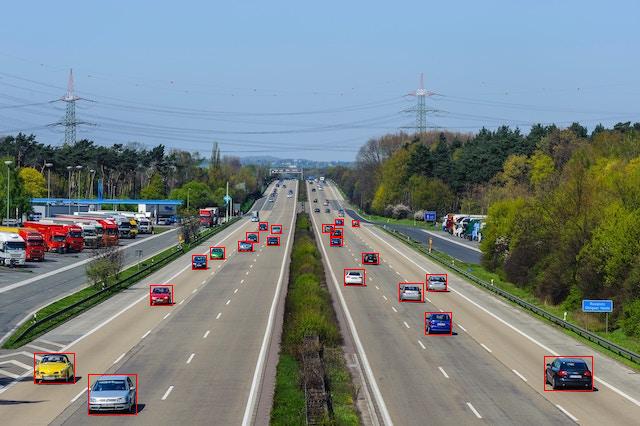
2 0.084375 0.866197 0.062500 0.075117
2 0.175000 0.924883 0.075000 0.093897
2 0.251563 0.693662 0.034375 0.049296
2 0.311719 0.616197 0.023438 0.035211
2 0.339844 0.595070 0.023438 0.030516
2 0.383594 0.577465 0.023438 0.028169
2 0.393750 0.557512 0.018750 0.025822
2 0.426563 0.565728 0.018750 0.023474
2 0.432031 0.538732 0.017188 0.021127
2 0.410938 0.531690 0.012500 0.021127
2 0.887500 0.875587 0.075000 0.084507
2 0.685937 0.759390 0.040625 0.053991
2 0.553125 0.652582 0.031250 0.037559
2 0.642188 0.687793 0.037500 0.042254
2 0.682031 0.663146 0.032813 0.039906
2 0.578125 0.606808 0.025000 0.025822
2 0.525000 0.565728 0.018750 0.023474
2 0.525781 0.546948 0.020313 0.023474
2 0.514062 0.536385 0.018750 0.021127
2 0.530469 0.521127 0.014063 0.018779
2 0.555469 0.524648 0.010937 0.016432
とりあえずpredictモードとvalモードを実行してみる
cars.yamlはcoco.yamlを参考に下記のように記入しています。namesは省略していますがcoco.yamlと同じ0~79番まで記載しています。
path: /Users/hinomaruc/Desktop/blog/dataset  # dataset root dir
train: images/train2017  # train images (relative to 'path') 128 images
val: ../aidetection_cars
test: ../aidetection_cars # test images (optional)

# Classes
names:
  0: person
  1: bicycle
  2: car
  3: motorcycle
  ・・・
79: toothbrushfrom ultralytics import YOLO
# 事前学習済みのモデルを読み込み(detectionモデルを使用)
model = YOLO('yolov8l.pt')
# predictモードを実行
results = model.predict(source="/Users/hinomaruc/Desktop/blog/dataset/aidetection_cars/alexander-schimmeck-W3MXYIfyxno-unsplash.jpg",
project="/Users/hinomaruc/Desktop/blog/dataset/yolov8/runs", # 出力先
name="cars", #フォルダ名
exist_ok=True,
classes=[2], #車のみ
show_conf=False,
show_labels=False,
line_width=1,
conf=0.25, # default=0.25
iou=0.7, # default=0.7
half=False, # default=False
save_txt=True, #アノテーションファイルの作成
save=True)
# valモードを実行 (predictの設定値と合わせる)
metrics = model.val(
data="/Users/hinomaruc/Desktop/blog/dataset/aidetection_cars/cars.yaml",
split='test', #testデータセットを使う。デフォルトはsplit='val'
conf=0.25, #default=0.001
iou=0.7, # default=0.6
half=False, # default=True
project="/Users/hinomaruc/Desktop/blog/dataset/yolov8/runs",
name="cars_val",
exist_ok=True,
save_json=True
)
image 1/1 /Users/hinomaruc/Desktop/blog/dataset/aidetection_cars/alexander-schimmeck-W3MXYIfyxno-unsplash.jpg: 448x640 20 cars, 3614.4ms
Speed: 3.0ms preprocess, 3614.4ms inference, 1.8ms postprocess per image at shape (1, 3, 640, 640)
Results saved to /Users/hinomaruc/Desktop/blog/dataset/yolov8/runs/cars
1 label saved to /Users/hinomaruc/Desktop/blog/dataset/yolov8/runs/cars/labels
Ultralytics YOLOv8.0.98 🚀 Python-3.7.16 torch-1.13.1 CPU
val: Scanning /Users/hinomaruc/Desktop/blog/dataset/aidetection_cars... 1 images
val: New cache created: /Users/hinomaruc/Desktop/blog/dataset/aidetection_cars.cache
                 Class     Images  Instances      Box(P          R      mAP50  m
                   all          1         21      0.952      0.952       0.97      0.745
                   car          1         21      0.952      0.952       0.97      0.745
Speed: 1.6ms preprocess, 3612.0ms inference, 0.0ms loss, 2.1ms postprocess per image
Saving /Users/hinomaruc/Desktop/blog/dataset/yolov8/runs/cars_val/predictions.json...
Results saved to /Users/hinomaruc/Desktop/blog/dataset/yolov8/runs/cars_val
上記detectの出力結果を確認すると、アノテーションした車両「21台」のうち「19台」は検知できているようです。
あれ?PrecisionとRecallは0.952ですね。20/21=0.952なのでvalの結果の期待値としてはgtから20台検知できているはずなのですが。。
詳しく見てみたら、predictとvalではなぜか出力される物体のconfの値が異なり、下記画像の車両はvalではconf:0.25以上の値で検知できているが、predictではconf:0.25より下の値で検出されていました。そのため、confの閾値を0.25で区切ると差異が出てしまっているようでした。
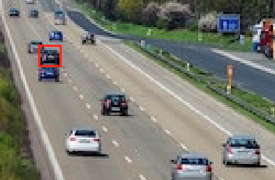
predictモードとvalモードは別物と考えていた方がいいのかも知れません。(私がパラメータを正しく設定できていないだけかも知れませんが)
predictの結果の確認方法
import pandas as pd
pd.DataFrame(zip(results[0].boxes.xyxy.numpy(),
                 results[0].boxes.conf.numpy()),columns=["bbox","conf"]
)bbox conf 0 [544.4082, 356.49774, 593.0547, 390.67163] 0.887329 1 [32.521423, 353.01245, 75.3817, 384.57086] 0.875159 2 [86.21228, 375.07538, 137.15167, 414.4007] 0.847157 3 [424.6319, 311.4176, 452.8156, 334.27344] 0.844650 4 [148.91875, 286.38452, 171.2354, 305.07507] 0.842991 5 [399.26355, 284.2237, 422.2928, 301.94818] 0.833451 6 [426.03323, 274.22357, 447.02347, 291.82318] 0.829037 7 [191.58607, 255.04633, 207.70403, 268.63104] 0.813592 8 [343.50732, 270.91913, 364.20984, 285.8813] 0.770575 9 [266.48495, 235.64572, 279.68393, 245.21661] 0.758867 10 [238.22737, 239.26065, 252.99614, 251.7778] 0.740608 11 [362.72745, 252.40863, 377.77103, 264.8819] 0.707603 12 [210.16402, 247.20618, 224.26207, 259.2638] 0.706635 13 [271.2323, 225.46227, 282.2926, 233.94029] 0.677294 14 [257.46368, 222.43932, 268.32355, 231.29396] 0.585063 15 [246.12085, 233.45856, 258.6018, 242.49963] 0.506521 16 [329.69385, 237.35547, 341.84363, 246.98514] 0.474564 17 [250.63904, 211.59245, 259.43732, 222.12303] 0.311763 18 [334.96863, 218.71829, 343.55322, 225.92667] 0.304380 19 [323.91455, 224.32875, 333.52576, 232.70958] 0.266846
/Users/hinomaruc/Desktop/blog/dataset/yolov8/runs/cars/以下に出力される検知結果の描画画像でもいいのですが、もう少し見やすいように独自に描画してみます。
import pandas as pd
from PIL import Image, ImageDraw, ImageFont

# 画像の読み込み
image = Image.open("/Users/hinomaruc/Desktop/blog/dataset/aidetection_cars/alexander-schimmeck-W3MXYIfyxno-unsplash.jpg")

# 描画オブジェクトの作成
draw = ImageDraw.Draw(image)

# フォントの設定
font = ImageFont.truetype('/System/Library/Fonts/ヒラギノ丸ゴ ProN W4.ttc', 6)

# 描画に情報をpredict結果から取得
pred_bbox = pd.DataFrame(zip(results[0].boxes.xyxy.numpy(),
                 results[0].boxes.conf.numpy()),columns=["bbox","conf"]
                 )

# ラベル描画用
offset=6

# bboxの読み込み
for line in pred_bbox.itertuples():

    # index
    idx=str(line.Index)

    # xyxyフォーマットなのでそのまま各変数に格納
    x1 = float(line.bbox[0])
    y1 = float(line.bbox[1])
    x2 = float(line.bbox[2])
    y2 = float(line.bbox[3])

    # 確信度
    conf=str(round(line.conf,2))

    # 描画テキスト。confも描画するとごちゃごちゃするのでインデックスだけにした
    label = idx

    # ラベルの背景色描画用
    text_bbox = draw.textbbox((x1 - offset, y1 - offset), label, font=font)
    text_bbox_x1, text_bbox_y1, text_bbox_x2, text_bbox_y2 = text_bbox
    draw.rectangle([text_bbox_x1, text_bbox_y1, text_bbox_x2, text_bbox_y2], fill="yellow")

    # ラベルの描画
    draw.text((x1 - offset, y1 - offset), label, fill="black",font=font)

    # bboxを描画する
    draw.rectangle([(x1, y1), (x2, y2)], outline="orange", width=1)

# 保存
image.save("labeled_image.jpg")
image.show()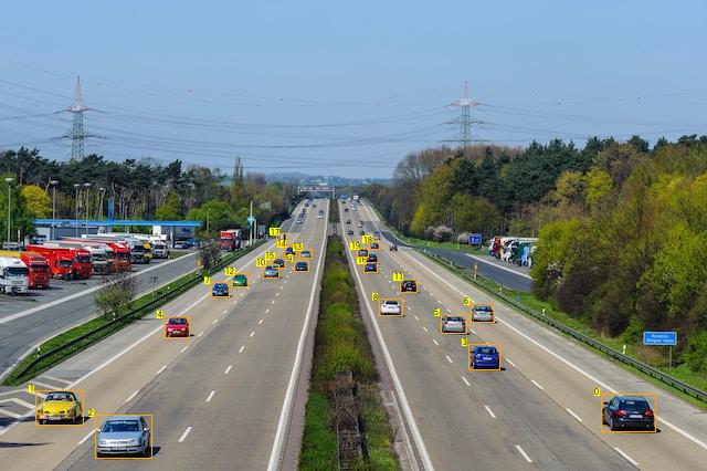
すっきりしていて見やすくなった、、と個人的に思っています 笑
valの結果の確認方法
import pandas as pd
df = pd.read_json('/Users/hinomaruc/Desktop/blog/dataset/yolov8/runs/cars_val/predictions.json')
val_bbox = df[df.category_id == 2].reset_index(drop=True)
val_bboximage_id category_id bbox score 0 alexander-schimmeck-W3MXYIfyxno-unsplash 2 [544.382, 356.461, 48.684, 34.182] 0.88665 1 alexander-schimmeck-W3MXYIfyxno-unsplash 2 [32.527, 352.972, 42.859, 31.574] 0.87902 2 alexander-schimmeck-W3MXYIfyxno-unsplash 2 [86.227, 375.07, 50.897, 39.315] 0.85367 3 alexander-schimmeck-W3MXYIfyxno-unsplash 2 [424.626, 311.408, 28.175, 22.847] 0.84988 4 alexander-schimmeck-W3MXYIfyxno-unsplash 2 [148.921, 286.382, 22.331, 18.689] 0.84884 5 alexander-schimmeck-W3MXYIfyxno-unsplash 2 [399.258, 284.189, 23.021, 17.734] 0.83969 6 alexander-schimmeck-W3MXYIfyxno-unsplash 2 [426.032, 274.202, 20.998, 17.608] 0.83607 7 alexander-schimmeck-W3MXYIfyxno-unsplash 2 [191.587, 255.053, 16.107, 13.573] 0.83522 8 alexander-schimmeck-W3MXYIfyxno-unsplash 2 [343.503, 270.91, 20.674, 14.952] 0.77880 9 alexander-schimmeck-W3MXYIfyxno-unsplash 2 [266.494, 235.631, 13.192, 9.567] 0.77739 10 alexander-schimmeck-W3MXYIfyxno-unsplash 2 [238.255, 239.263, 14.738, 12.482] 0.77373 11 alexander-schimmeck-W3MXYIfyxno-unsplash 2 [210.173, 247.191, 14.089, 12.033] 0.72787 12 alexander-schimmeck-W3MXYIfyxno-unsplash 2 [362.733, 252.381, 15.034, 12.477] 0.71466 13 alexander-schimmeck-W3MXYIfyxno-unsplash 2 [271.221, 225.438, 11.097, 8.464] 0.69139 14 alexander-schimmeck-W3MXYIfyxno-unsplash 2 [257.476, 222.43, 10.829, 8.842] 0.60926 15 alexander-schimmeck-W3MXYIfyxno-unsplash 2 [246.107, 233.452, 12.538, 9.018] 0.54828 16 alexander-schimmeck-W3MXYIfyxno-unsplash 2 [329.688, 237.325, 12.164, 9.639] 0.53467 17 alexander-schimmeck-W3MXYIfyxno-unsplash 2 [334.938, 218.695, 8.633, 7.213] 0.37053 18 alexander-schimmeck-W3MXYIfyxno-unsplash 2 [250.624, 211.607, 8.802, 10.478] 0.35711 19 alexander-schimmeck-W3MXYIfyxno-unsplash 2 [323.902, 224.298, 9.58, 8.408] 0.30688 20 alexander-schimmeck-W3MXYIfyxno-unsplash 2 [330.884, 228.934, 11.398, 10.173] 0.28005
やはりvalの方が1件多く検知できているようです。image_id=20がpredictモードで出てこなかった車両のようです。
bboxを描画したいと思います。
/Users/hinomaruc/Desktop/blog/dataset/yolov8/runs/cars_val/val_batch0_pred.jpg にもvalでの検知結果が確認できますが、物体の描画件数が15件で足切りされていると思われるので参考情報とした方がいいと考えます。
出力結果の1つであるval_batch0_pred.jpgですが、最大15個しか検知結果を表示しないように制御しているようです。詳細:val.py#L222。そして、もしかしたらconfも0.25で足切りされているかも? 詳細:plotting.py#L372
引用: https://www.hinomaruc.com/check-the-metrics-of-object-detection-results-using-yolov8-val-mode/#toc10
# valの結果
import pandas as pd
from PIL import Image, ImageDraw, ImageFont

# 画像の読み込み
image = Image.open("/Users/hinomaruc/Desktop/blog/dataset/aidetection_cars/alexander-schimmeck-W3MXYIfyxno-unsplash.jpg")

# 描画オブジェクトの作成
draw = ImageDraw.Draw(image)

# フォントの設定
font = ImageFont.truetype('/System/Library/Fonts/ヒラギノ丸ゴ ProN W4.ttc', 6)

# ラベル描画用
offset=6

# bboxの読み込み
for line in val_bbox.itertuples():

    # index
    idx=str(line.Index)

    # xywhフォーマットのようなので、xyxyに変換する
    x1 = float(line.bbox[0])
    y1 = float(line.bbox[1])
    width = float(line.bbox[2])
    height = float(line.bbox[3])
    x2 = x1 + width
    y2 = y1 + height

    # 確信度
    conf=str(round(line.score,2))

    # 描画テキスト。confも描画するとごちゃごちゃするのでインデックスだけにした
    label = idx

    # ラベルの背景色描画用
    text_bbox = draw.textbbox((x1 - offset, y1 - offset), label, font=font)
    text_bbox_x1, text_bbox_y1, text_bbox_x2, text_bbox_y2 = text_bbox
    draw.rectangle([text_bbox_x1, text_bbox_y1, text_bbox_x2, text_bbox_y2], fill="yellow")

    # ラベルの描画
    draw.text((x1 - offset, y1 - offset), label, fill="black",font=font)

    # bboxを描画する
    draw.rectangle([(x1, y1), (x2, y2)], outline="red", width=1)

# 保存
image.save("labeled_image.jpg")
image.show()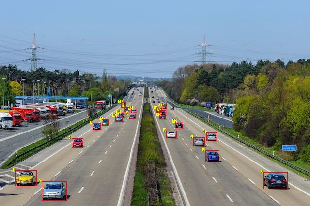
特定の領域内のみを対象に物体検知の結果を描画する
かなり長くなってきましたが、本記事で一番やりたかったことになります。
レイアウトごとにポリゴンを描画する必要があるので、不特定多数の画像というよりはどこかにカメラを固定で設置して同じ座標に対して検知するイメージになります。
まずは特定領域になるポリゴンを決めて、領域内の検知物体のみに限定します。
その次に限定した検知物体のみで精度を求めてみようと思います。
必要な処理を関数化
まずはbbox描画処理と特定エリア内のbboxを抽出する処理を使いまわせるように関数化しておきます。
どういう風に作ろうか少し悩みました。draw_bboxの方は複数エリアを描画できるようにしていますが、get_bbox_inside_polygonでは1つのエリアしか対応していません。
get_bbox_inside_polygonが1エリアのみしか対応しないようにしたのは、処理が複雑になりそうだったのと、抽出に関してはエリアごとにbboxをカウントしたい需要があるかなと考えエリアの数だけループを複数回実行すればいいかなと思い立ったためです 笑
画像は固定で読み込んでいるので必要に応じて変更する必要があります。
"""
    Displays bounding boxes on the specified image. polygon_list displays input polygon area.

    Arguments:
    - bbox_list_xyxy: List of bounding boxes in xyxy format.
    - bbox_color: Set the color of bbox lines. Default is Orange
    - polygon_list: List of polygons representing input polygon areas. (Optional)
"""
def draw_bbox(bbox_list_xyxy,bbox_color="orange",polygon_list=None):
    from PIL import Image, ImageDraw, ImageFont

    # 画像の読み込み
    image = Image.open("/Users/hinomaruc/Desktop/blog/dataset/aidetection_cars/alexander-schimmeck-W3MXYIfyxno-unsplash.jpg")

    # 描画オブジェクトの作成
    draw = ImageDraw.Draw(image)

    # フォントの設定
    font = ImageFont.truetype('/System/Library/Fonts/ヒラギノ丸ゴ ProN W4.ttc', 6)

    # ラベル描画用
    offset=6

    # 検知するエリアの指定と描画
    if polygon_list is not None:
        if isinstance(polygon_list[0], tuple):
            draw.polygon(polygon_list, outline="yellow", fill=None)
        else:
            for apolygon in polygon_list:
                #polygon_points = apolygon # [(5,415), (55,323), (140,268), (280,268), (265,415)]
                draw.polygon(apolygon, outline="yellow", fill=None)

    # bboxの読み込み
    for idx,bbox_xyxy in enumerate(bbox_list_xyxy):

        # xyxyフォーマット
        x1 = float(bbox_xyxy[0])
        y1 = float(bbox_xyxy[1])
        x2 = float(bbox_xyxy[2])
        y2 = float(bbox_xyxy[3])

        # 描画テキスト。confも描画するとごちゃごちゃするのでインデックスだけにした
        label = str(idx)

        # ラベルの背景色描画用
        text_bbox = draw.textbbox((x1 - offset, y1 - offset), label, font=font)
        text_bbox_x1, text_bbox_y1, text_bbox_x2, text_bbox_y2 = text_bbox
        draw.rectangle([text_bbox_x1, text_bbox_y1, text_bbox_x2, text_bbox_y2], fill="yellow")

        # ラベルの描画
        draw.text((x1 - offset, y1 - offset), label, fill="black",font=font)

        # bboxを描画する
        draw.rectangle([(x1, y1), (x2, y2)], outline=bbox_color, width=1)

    # 保存
    image.save("labeled_image.jpg")
    # 表示
    image.show()
"""
Finds bounding boxes that are inside a given polygon.

Arguments:
- polygon: List of points defining the area polygon.
- bbox_list_xyxy: List of bounding boxes in xyxy format.
- conf_list: List of confidence values for each bounding box. (Optional)

Returns:
- bbox_inside_poly: List of bounding boxes that are inside the polygon.
- conf_inside_poly: List of confidence values corresponding to the bounding boxes. (Empty if conf_list is None)
"""
def get_bbox_inside_polygon(polygon, bbox_list_xyxy, conf_list=None):
    from shapely.geometry import Point, Polygon
    from rtree import index

    # shapelyのポリゴンの作成
    area_polygon = Polygon(polygon)

    # R-tree indexの作成
    idx = index.Index()

    # R-tree indexにbbox(xyxyフォーマット)をインサート
    for i, bbox in enumerate(bbox_list_xyxy):
        idx.insert(i, bbox)

    bbox_inside_poly = []
    conf_inside_poly = []
    mode = "center"  # center or restrict

    # エリア内のバウンディングボックスを抽出
    for i in idx.intersection(area_polygon.bounds):
        bbox = bbox_list_xyxy[i]

        # centerモードはbboxの中心点がエリア内に位置するか判定する
        if mode == 'center':
            center_x = (bbox[0] + bbox[2]) / 2
            center_y = (bbox[1] + bbox[3]) / 2
            bbox_polygon = Point(center_x, center_y)
        # strictモードはbboxの左上から右下までが厳密にエリア内かどうかを判定する
        else:
            bbox_polygon = Polygon([(bbox[0], bbox[1]), (bbox[0], bbox[3]), (bbox[2], bbox[3]), (bbox[2], bbox[1])])

        # 抽出結果を格納
        if area_polygon.contains(bbox_polygon):
            bbox_inside_poly.append(bbox)

            if conf_list is not None and len(conf_list) == len(bbox_list_xyxy):
                conf_inside_poly.append(conf_list[i])

    return bbox_inside_poly, conf_inside_poly
1つのエリア内で検知した物体を描画
左側のレーンの下の方だけ検知したい場合を想定しています。
# 描画に情報をpredict結果から取得
pred_bbox = results[0].boxes.xyxy
pred_conf = results[0].boxes.conf
area1=[(5, 415), (55, 323), (140, 268), (280, 268), (265, 415)]
pred_bbox_filtered,pred_conf_filtered = get_bbox_inside_polygon(area1, pred_bbox,pred_conf)

# 抽出したbboxとconfを表示
for row in zip(pred_bbox_filtered,pred_conf_filtered):
    print(row)

# 抽出したbboxとエリアを描画する
draw_bbox(pred_bbox_filtered,polygon_list=area1)(tensor([ 32.5214, 353.0125, 75.3817, 384.5709]), tensor(0.8752)) (tensor([ 86.2123, 375.0754, 137.1517, 414.4007]), tensor(0.8472)) (tensor([148.9187, 286.3845, 171.2354, 305.0751]), tensor(0.8430))
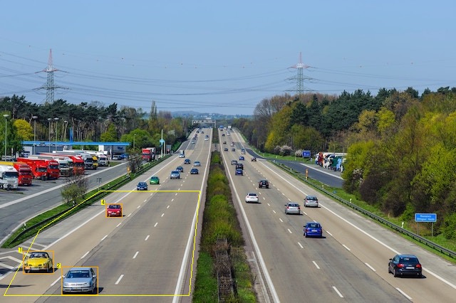
出来ました。次は右側のレーンにもエリアを作成してみます。
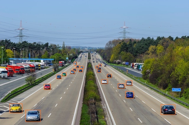
複数のエリア内で検知した物体を描画
右側のレーンの大部分にもエリアを作成してみました。
左側のレーンのエリアはそのまま指定しています。
# 描画に情報をpredict結果から取得
pred_bbox = results[0].boxes.xyxy
pred_conf = results[0].boxes.conf
area1=[(5, 415), (55, 323), (140, 268), (280, 268), (265, 415)]
area2=[(310,215),(360,215),(630,395),(360,395)]
area_list = [area1, area2]

pred_bbox_filtered = []
pred_conf_filtered = []

# 複数エリアからbboxを抽出する
for area in area_list:
    area_bbox, area_conf = get_bbox_inside_polygon(area, pred_bbox, pred_conf)
    pred_bbox_filtered.extend(area_bbox)
    pred_conf_filtered.extend(area_conf)

# 抽出したbboxとconfを表示
for row in zip(pred_bbox_filtered,pred_conf_filtered):
    print(row)

# 抽出したbboxとエリアを描画する
draw_bbox(pred_bbox_filtered,polygon_list=area_list)(tensor([ 32.5214, 353.0125, 75.3817, 384.5709]), tensor(0.8752)) (tensor([ 86.2123, 375.0754, 137.1517, 414.4007]), tensor(0.8472)) (tensor([148.9187, 286.3845, 171.2354, 305.0751]), tensor(0.8430)) (tensor([544.4082, 356.4977, 593.0547, 390.6716]), tensor(0.8873)) (tensor([424.6319, 311.4176, 452.8156, 334.2734]), tensor(0.8447)) (tensor([399.2635, 284.2237, 422.2928, 301.9482]), tensor(0.8335)) (tensor([426.0332, 274.2236, 447.0235, 291.8232]), tensor(0.8290)) (tensor([343.5073, 270.9191, 364.2098, 285.8813]), tensor(0.7706)) (tensor([362.7274, 252.4086, 377.7710, 264.8819]), tensor(0.7076)) (tensor([329.6938, 237.3555, 341.8436, 246.9851]), tensor(0.4746)) (tensor([334.9686, 218.7183, 343.5532, 225.9267]), tensor(0.3044)) (tensor([323.9146, 224.3288, 333.5258, 232.7096]), tensor(0.2668))
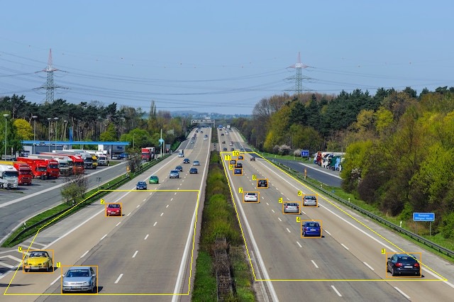
いい感じですね。きちんとエリア内のみbboxが表示されています。次はエリア内のbboxを対象に精度を算出してみます。
ちなみにエリア内で検知した台数を取得したい場合はbboxの件数を取得すればOKです。len(pred_bbox_filtered)を実行すると12という結果が返ってきます。
len(pred_bbox_filtered)はarea1とarea2内の検知物体の合算件数です。エリアごとの台数を取得したい場合は、下記コードのarea_bboxの長さをそれぞれ取得する必要があります。
複数エリアからbboxを抽出する
for area in area_list:
area_bbox, area_conf = get_bbox_inside_polygon(area, pred_bbox, pred_conf)
pred_bbox_filtered.extend(area_bbox)
pred_conf_filtered.extend(area_conf)
特定の領域内のみを対象に物体検知の精度を求める
指定したエリア内を対象にAverage Precisionを計算して見ようと思います。自分で全て計算してみようと思いましたが大変なので今回は「review_object_detection_metrics」というツールと「TorchMetrics」というライブラリを試してみたいと思います。
今回のケースでは全部で14台の車両がエリア1とエリア2内に存在していて、検知出来ているのはそのうち12台のみという結果に対する精度を求めることになります。
まずはGround Truthを設定したエリア内のみにフィルタリングする
精度を求めるためには正解ラベルの情報が必要です。設定したエリア内に存在する正解ラベルを抽出もしくは作成します。
最初から領域が決められていればフィルタリングせずに該当箇所だけアノテーションしたファイルを作成するでも問題ありません。
xywhnフォーマットからxyxyフォーマットに変換する処理は繰り返す使うことになると思うので関数化してもいいかも。
from PIL import Image

gt_list_xyxy=[]
gt_bbox_filtered=[]

# 画像の読み込み (サイズを取得するためだけ)
image = Image.open("/Users/hinomaruc/Desktop/blog/dataset/aidetection_cars/alexander-schimmeck-W3MXYIfyxno-unsplash.jpg")

# アノテーションしたファイルの読み込み
with open("/Users/hinomaruc/Desktop/blog/dataset/aidetection_cars/alexander-schimmeck-W3MXYIfyxno-unsplash.txt", "r") as file:
    lines = file.readlines()

# YOLOフォーマットtxtの読み込み
for line in lines:

    line = line.strip().split(" ")

    # LabelImgで作成したので、class + xywhnフォーマットになっている
    class_index = int(line[0]) # クラス番号
    x_normalized = float(line[1]) # 標準化済みx
    y_normalized = float(line[2]) # 標準化済みy
    width_normalized = float(line[3]) # 標準化済みwidth
    height_normalized = float(line[4]) # 標準化済みheight

    # 標準化xywhをピクセル値に変換する
    width, height = image.size # 画像サイズの取得
    x_pixel = int(x_normalized * width)
    y_pixel = int(y_normalized * height)
    width_pixel = int(width_normalized * width)
    height_pixel = int(height_normalized * height)

    # xyxyフォーマットに変換
    x1 = x_pixel - (width_pixel // 2)
    y1 = y_pixel - (height_pixel // 2)
    x2 = x_pixel + (width_pixel // 2)
    y2 = y_pixel + (height_pixel // 2)

    gt_list_xyxy.append([x1,y1,x2,y2])

area1=[(5, 415), (55, 323), (140, 268), (280, 268), (265, 415)]
area2=[(310,215),(360,215),(630,395),(360,395)]
area_list = [area1, area2]

# 複数エリアからbboxを抽出する
for area in area_list:
    area_bbox, _ = get_bbox_inside_polygon(area, gt_list_xyxy)
    gt_bbox_filtered.extend(area_bbox)

print(gt_bbox_filtered)

# 抽出したbboxとエリアを描画する
draw_bbox(gt_bbox_filtered,bbox_color="red",polygon_list=area_list)[[34, 353, 74, 383], [88, 374, 136, 414], [150, 285, 172, 305], [544, 356, 592, 390], [425, 312, 451, 334], [344, 269, 364, 285], [399, 283, 423, 301], [426, 274, 446, 290], [362, 253, 378, 263], [330, 237, 342, 245], [330, 228, 342, 236], [322, 224, 334, 232], [335, 219, 343, 225], [352, 220, 358, 226]]

14つ残りました。想定通りです。
review_object_detection_metrics利用して精度を求める
review_object_detection_metricsはGUIツールになります。23年5月現在、CUI機能は未対応です。
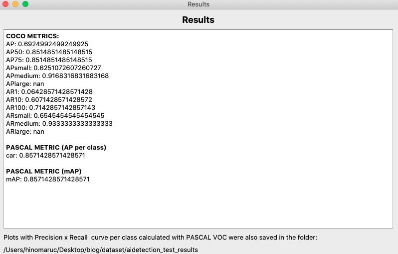
使用したアノテーションデータは下記になります。detection.txtはpred_bbox_filteredとpred_conf_filteredから作成し、ground truth.txtはlabelimgから必要のないラベルを除外して作成しました。
pred_list_xywhn = []

for row in zip(pred_bbox_filtered, pred_conf_filtered):
    x1, y1, x2, y2 = row[0]
    width = x2 - x1
    height = y2 - y1
    class_index = 2
    x_center_normalized = (x1 + x2) / 2 / image.width
    y_center_normalized = (y1 + y2) / 2 / image.height
    width_normalized = width / image.width
    height_normalized = height / image.height
    conf = row[1]

    pred_list_xywhn.append([class_index, conf, x_center_normalized, y_center_normalized, width_normalized, height_normalized])

# pred_list_xywhnをtxtファイルに出力する
output_array = np.array(pred_list_xywhn)
output_file_path = 'detection.txt'
np.savetxt(output_file_path, output_array, fmt=['%.0f', '%.4f', '%.4f', '%.4f', '%.4f', '%.4f'])- detection.txt (label,conf,x,y,w,h) normalized
2 0.8752 0.0843 0.8657 0.0670 0.0741
2 0.8472 0.1745 0.9266 0.0796 0.0923
2 0.8430 0.2501 0.6942 0.0349 0.0439
2 0.8873 0.8886 0.8770 0.0760 0.0802
2 0.8447 0.6855 0.7579 0.0440 0.0537
2 0.8335 0.6418 0.6880 0.0360 0.0416
2 0.8290 0.6821 0.6644 0.0328 0.0413
2 0.7706 0.5529 0.6535 0.0323 0.0351
2 0.7076 0.5785 0.6071 0.0235 0.0293
2 0.4746 0.5246 0.5685 0.0190 0.0226
2 0.3044 0.5301 0.5219 0.0134 0.0169
2 0.2668 0.5136 0.5364 0.0150 0.0197
- ground truth.txt (label,x,y,w,h) normalized
2 0.084375 0.866197 0.062500 0.075117
2 0.175000 0.924883 0.075000 0.093897
2 0.251563 0.693662 0.034375 0.049296
2 0.887500 0.875587 0.075000 0.084507
2 0.685937 0.759390 0.040625 0.053991
2 0.553125 0.652582 0.031250 0.037559
2 0.642188 0.687793 0.037500 0.042254
2 0.682031 0.663146 0.032813 0.039906
2 0.578125 0.606808 0.025000 0.025822
2 0.525000 0.565728 0.018750 0.023474
2 0.525781 0.546948 0.020313 0.023474
2 0.514062 0.536385 0.018750 0.021127
2 0.530469 0.521127 0.014063 0.018779
2 0.555469 0.524648 0.010937 0.016432
中サイズの物体に対する精度(APmedium)は0.9とかなり良いですが、小サイズの物体に対する精度(APsmall)は0.625と低いことがすぐに分かります。
大サイズの物体(APlarge)はnanになっているので、今回のデータセットでは存在しないようです。
TorchMetricsを利用して精度を求める
TorchMetricsで精度を求めるのに必要な情報を取得します。分かりやすいのでpandasでまとめました。
review_object_detection_metricsはxywhnフォーマットでしたが、TorchMetricsでは仕様のためxyxyフォーマットに統一しています。
ただ、引数でbox_formatという項目があり、 ["xyxy", "xywh", "cxcywh"]のどれかを選択できるようでした。もしかしたらxywhフォーマットでも動作するのかも知れません。
Predicted boxes and targets have to be in Pascal VOC format (xmin-top left, ymin-top left, xmax-bottom right, ymax-bottom right).
引用: https://torchmetrics.readthedocs.io/en/stable/detection/mean_average_precision.html
後ほど確認出来ますが、フォーマット間で変換処理を実行しているためかreview_object_detection_metricsとTorchMetricsの結果に若干の誤差が生じています。とはいえAP@50だと両方とも同じAP値だったので問題なさそうな気がしています。
また、TorchMetricsはpycocotoolsのmAPの計算方法に準じているらしいので、結果に関しては信頼してもいいのではないかと思います。
This metric is following the mAP implementation of pycocotools, a standard implementation for the mAP metric for object detection.
引用: https://torchmetrics.readthedocs.io/en/stable/detection/mean_average_precision.html
それではTorchMetricsを使ってみます。
(venv-yolov8) pip install torchmetrics
Collecting torchmetrics
  Downloading torchmetrics-0.11.4-py3-none-any.whl (519 kB)
     ━━━━━━━━━━━━━━━━━━━━━━━━━━━━━━━━━━━━━━━ 519.2/519.2 kB 8.8 MB/s eta 0:00:00
Requirement already satisfied: numpy>=1.17.2 in ./venv-yolov8/lib/python3.7/site-packages (from torchmetrics) (1.21.6)
Requirement already satisfied: torch>=1.8.1 in ./venv-yolov8/lib/python3.7/site-packages (from torchmetrics) (1.13.1)
Requirement already satisfied: packaging in ./venv-yolov8/lib/python3.7/site-packages (from torchmetrics) (23.1)
Requirement already satisfied: typing-extensions in ./venv-yolov8/lib/python3.7/site-packages (from torchmetrics) (4.5.0)
Installing collected packages: torchmetrics
Successfully installed torchmetrics-0.11.4
data = []
for row in zip(pred_bbox_filtered, pred_conf_filtered):
    bbox = np.array(row[0])
    conf = np.array(row[1])
    data.append([bbox, conf])

df_pred_bbox_filtered = pd.DataFrame(data, columns=['pred_bbox', 'conf'])
df_pred_bbox_filtered["label"] = 2 # carを指定

print(df_pred_bbox_filtered)
                                       pred_bbox        conf  label
0     [32.521423, 353.01245, 75.3817, 384.57086]   0.8751586      2
1     [86.21228, 375.07538, 137.15167, 414.4007]    0.847157      2
2    [148.91875, 286.38452, 171.2354, 305.07507]   0.8429913      2
3     [544.4082, 356.49774, 593.0547, 390.67163]   0.8873292      2
4      [424.6319, 311.4176, 452.8156, 334.27344]   0.8446502      2
5     [399.26355, 284.2237, 422.2928, 301.94818]   0.8334514      2
6   [426.03323, 274.22357, 447.02347, 291.82318]   0.8290367      2
7    [343.50732, 270.91913, 364.20984, 285.8813]  0.77057505      2
8    [362.72745, 252.40863, 377.77103, 264.8819]  0.70760274      2
9   [329.69385, 237.35547, 341.84363, 246.98514]  0.47456363      2
10  [334.96863, 218.71829, 343.55322, 225.92667]   0.3043804      2
11  [323.91455, 224.32875, 333.52576, 232.70958]   0.2668459      2
df_gt_bbox_filtered = pd.DataFrame({"gt_bbox": gt_bbox_filtered})
df_gt_bbox_filtered["label"] = 2 # carを指定

print(df_gt_bbox_filtered)
                 gt_bbox  label
0     [34, 353, 74, 383]      2
1    [88, 374, 136, 414]      2
2   [150, 285, 172, 305]      2
3   [544, 356, 592, 390]      2
4   [425, 312, 451, 334]      2
5   [344, 269, 364, 285]      2
6   [399, 283, 423, 301]      2
7   [426, 274, 446, 290]      2
8   [362, 253, 378, 263]      2
9   [330, 237, 342, 245]      2
10  [330, 228, 342, 236]      2
11  [322, 224, 334, 232]      2
12  [335, 219, 343, 225]      2
13  [352, 220, 358, 226]      2
材料は揃ったので精度を求めてみます.
import torch
from torchmetrics.detection.mean_ap import MeanAveragePrecision
from pprint import pprint

preds = [
dict(
    boxes=torch.tensor([np.array(bbox) for bbox in df_pred_bbox_filtered["pred_bbox"].values]),
    scores=torch.tensor([conf.item() for conf in df_pred_bbox_filtered["conf"]]),
    labels=torch.tensor(df_pred_bbox_filtered["label"].tolist()),
    )
]

target = [
    dict(
    boxes=torch.tensor([np.array(bbox) for bbox in df_gt_bbox_filtered["gt_bbox"].values]),
    labels=torch.tensor(df_gt_bbox_filtered["label"].tolist()),
    )
]

metric = MeanAveragePrecision(iou_type="bbox",compute_on_cpu=True)
metric.update(preds, target)
pprint(metric.compute())
{'map': tensor(0.6089),
 'map_50': tensor(0.8515),
 'map_75': tensor(0.7066),
 'map_large': tensor(-1.),
 'map_medium': tensor(0.8554),
 'map_per_class': tensor(-1.),
 'map_small': tensor(0.5415),
 'mar_1': tensor(0.0643),
 'mar_10': tensor(0.5357),
 'mar_100': tensor(0.6143),
 'mar_100_per_class': tensor(-1.),
 'mar_large': tensor(-1.),
 'mar_medium': tensor(0.8667),
 'mar_small': tensor(0.5455)}
自分で実装するより遥かに楽ですね 笑
まとめ
かなり長くなってしまいましたが、特定のエリア内の物体検知件数と精度を求めることが出来ました。
ここまで試みてきたことで実業務では大抵のことが出来るようになったのではないでしょうか。
次は物体検知APIの作成をやってみようと思います。画像をサーバー側に渡しJSON形式で検知結果を返却するといった処理を想定して作ってみようと思います。