今回は前回の続きでランダムフォーレスト(random forest)のパラメータチューニングをベイズ最適化(Bayesian Optimization)で行いたいと思います。
色々と調べている中、ベイズ最適化はグリッドサーチのように総当たりで最適なパラメータを発掘するのではなく、ある程度当たりをつけながら最適なパラメータを探索してくれる手法というイメージを持ちました。
ランダムフォーレストのベイズ最適化はこちらのコードを参考にしました。
それではやっていきます。
Bayesian Optimizationライブラリのインストール
GitHubで公開してくださっている方がいるので活用させていただきます。
基本ReadMeの通りやっていけばOKです。
まずは、
If you are using scipy>1.8.x, please install directly from this branch: e.g. pip install git+https://github.com/fmfn/BayesianOptimization
という記載があるので、scipyのバージョンを確認します。
import scipy
scipy.__version__'1.8.1'
1.8以上だったので、注意書きの通り直接GitHubのブランチからインストールします。
# BayesianOptimizationのインストール
pip install git+https://github.com/fmfn/BayesianOptimizationCollecting git+https://github.com/fmfn/BayesianOptimization Cloning https://github.com/fmfn/BayesianOptimization to /private/var/folders/n0/ft3172td6v70d6klgt216_3r0000gn/T/pip-req-build-la4bz5a3 Running command git clone --filter=blob:none --quiet https://github.com/fmfn/BayesianOptimization /private/var/folders/n0/ft3172td6v70d6klgt216_3r0000gn/T/pip-req-build-la4bz5a3 Resolved https://github.com/fmfn/BayesianOptimization to commit 1aaa255591aa4c5514bf3ea5ed3b0270f6cce575 Preparing metadata (setup.py) ... done ・・・省略・・・ Successfully built bayesian-optimization Installing collected packages: bayesian-optimization Successfully installed bayesian-optimization-1.2.0
評価指標
住宅IdごとのSalePrice(販売価格)を予測するコンペです。
評価指標は予測SalePriceと実測SalePriceの対数を取ったRoot-Mean-Squared-Error(RMSE)の値のようです。

ランダムフォーレスト分析
分析用データの準備
事前に欠損値処理や特徴量エンジニアリングを実施してデータをエクスポートしています。
本記事と同じ結果にするためには事前に下記記事を確認してデータを用意してください。
(その3-2) エイムズの住宅価格のデータセットのデータ加工①
(その3-3) エイムズの住宅価格のデータセットのデータ加工②
学習用データとスコア付与用データの読み込み
import pandas as pd
import numpy as np
# エイムズの住宅価格のデータセットの訓練データとテストデータを読み込む
df = pd.read_csv("/Users/hinomaruc/Desktop/blog/dataset/ames/ames_train.csv")
df_test = pd.read_csv("/Users/hinomaruc/Desktop/blog/dataset/ames/ames_test.csv")
df.head()
Id LotFrontage LotArea LotShape Utilities LandSlope OverallQual OverallCond MasVnrArea ExterCond ... SaleType_New SaleType_Oth SaleType_WD SaleCondition_Abnorml SaleCondition_AdjLand SaleCondition_Alloca SaleCondition_Family SaleCondition_Normal SaleCondition_Partial SalePrice 0 1 65.0 8450 3.0 3.0 2.0 7 5 196.0 2.0 ... 0.0 0.0 1.0 0.0 0.0 0.0 0.0 1.0 0.0 208500 1 2 80.0 9600 3.0 3.0 2.0 6 8 0.0 2.0 ... 0.0 0.0 1.0 0.0 0.0 0.0 0.0 1.0 0.0 181500 2 3 68.0 11250 2.0 3.0 2.0 7 5 162.0 2.0 ... 0.0 0.0 1.0 0.0 0.0 0.0 0.0 1.0 0.0 223500 3 4 60.0 9550 2.0 3.0 2.0 7 5 0.0 2.0 ... 0.0 0.0 1.0 1.0 0.0 0.0 0.0 0.0 0.0 140000 4 5 84.0 14260 2.0 3.0 2.0 8 5 350.0 2.0 ... 0.0 0.0 1.0 0.0 0.0 0.0 0.0 1.0 0.0 250000 5 rows × 335 columns
# 描画設定
from IPython.display import HTML
import seaborn as sns
from matplotlib import ticker
import matplotlib.pyplot as plt
sns.set_style("whitegrid")
from matplotlib import rcParams
rcParams['font.family'] = 'Hiragino Sans' # Macの場合
#rcParams['font.family'] = 'Meiryo' # Windowsの場合
#rcParams['font.family'] = 'VL PGothic' # Linuxの場合
rcParams['xtick.labelsize'] = 12       # x軸のラベルのフォントサイズ
rcParams['ytick.labelsize'] = 12       # y軸のラベルのフォントサイズ
rcParams['axes.labelsize'] = 18        # ラベルのフォントとサイズ
rcParams['figure.figsize'] = 18,8      # 画像サイズの変更(inch)
ランダムフォーレストに使用する変数を選ぶ
とりあえず全て突っ込んでみます
ランダムフォーレストで学習を実施 (ベイズ最適化によるパラメータチューニング)
# 説明変数と目的変数を指定

# 学習データ
X_train = df.drop(["Id","SalePrice"],axis=1)
Y_train = df["SalePrice"] # 販売価格

# テストデータ
X_test = df_test.drop(["Id"],axis=1)
# ベイズ最適化
from bayes_opt import BayesianOptimization
# ランダムフォーレスト
from sklearn.ensemble import RandomForestRegressor
# 評価指標 (どっちも試してよい結果を採用しようと思います。)
from sklearn.metrics import mean_squared_error
from sklearn.metrics import mean_squared_log_error
# 交差検証 (https://scikit-learn.org/stable/modules/generated/sklearn.model_selection.cross_validate.html)
from sklearn.model_selection import cross_validate"""
RandomForest(交差検証あり)
"""
def random_forest_cv(X, y, scoring, **kwargs):
regr = RandomForestRegressor(random_state=1414, **kwargs)
cv_results = cross_validate(regr, X, y
, scoring = scoring # "neg_mean_squared_error,neg_root_mean_squared_error,neg_mean_squared_log_errorで検証してみる
, cv = 5 # 交差検証数 5-fold
, verbose = 2 # ログレベル
, n_jobs = -1 # 並列実行数 -1:全プロセッサ利用
)
return cv_results['test_score'].mean()random_forest_cv(X_train,Y_train,'neg_mean_squared_error')[Parallel(n_jobs=-1)]: Using backend LokyBackend with 4 concurrent workers. [Parallel(n_jobs=-1)]: Done 5 out of 5 | elapsed: 6.4s finished -882864106.3749046
"""
Wrapper of RandomForest cross validation.
"""
def bayesian_optimise_rf(X, y, n_iter = 100):

    def rf_crossval(n_estimators, max_features,min_samples_split):
        return random_forest_cv(
            X = X,
            y = y,
            scoring='neg_mean_squared_error',
            n_estimators = int(n_estimators),
            max_features = max(min(max_features, 0.999), 1e-3), #
            min_samples_split = int(min_samples_split)
        )

    optimizer = BayesianOptimization(
        f = rf_crossval, # black box function (最適化したい関数)
        pbounds = {
            "n_estimators" : (10, 400),
            "max_features" : (0.1, 0.999),
            "min_samples_split" : (2,50)
        }
    )

    optimizer.maximize(n_iter = n_iter)

    print("Final result:", optimizer.max)
bayesian_optimise_rf(X_train,Y_train)
|   iter    |  target   | max_fe... | min_sa... | n_esti... |
-------------------------------------------------------------

[Parallel(n_jobs=-1)]: Using backend LokyBackend with 4 concurrent workers.
[Parallel(n_jobs=-1)]: Done   5 out of   5 | elapsed:   10.1s finished
[Parallel(n_jobs=-1)]: Using backend LokyBackend with 4 concurrent workers.

| 1         | -9.827e+0 | 0.2725    | 38.92     | 354.3     |

[Parallel(n_jobs=-1)]: Done   5 out of   5 | elapsed:    5.4s finished
[Parallel(n_jobs=-1)]: Using backend LokyBackend with 4 concurrent workers.

| 2         | -8.858e+0 | 0.4678    | 24.19     | 227.6     |

・・・省略・・・

Final result: {'target': -809969600.8095932, 'params': {'max_features': 0.3814608551637303, 'min_samples_split': 5.840239834845827, 'n_estimators': 193.56063863177957}}

[Parallel(n_jobs=-1)]: Done   5 out of   5 | elapsed:    3.1s finished
ベイズ最適化は少ない試行の中で最大のパフォーマンスを出そうとする手法のようなので、最終的にはグリッドサーチやランダムサーチで総当たりで最適化した結果と似てくるようです。
# https://scikit-learn.org/stable/modules/generated/sklearn.ensemble.RandomForestRegressor.html
from sklearn.ensemble import RandomForestRegressor

# モデル作成
regr = RandomForestRegressor(random_state=1414,max_features=0.3814608551637303,min_samples_split=6,n_estimators=193)

# フィット
regr.fit(X_train,Y_train)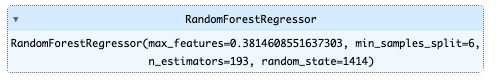
# モデルパラメータ一覧
regr.get_params()
    {'bootstrap': True,
     'ccp_alpha': 0.0,
     'criterion': 'squared_error',
     'max_depth': None,
     'max_features': 0.3814608551637303,
     'max_leaf_nodes': None,
     'max_samples': None,
     'min_impurity_decrease': 0.0,
     'min_samples_leaf': 1,
     'min_samples_split': 6,
     'min_weight_fraction_leaf': 0.0,
     'n_estimators': 193,
     'n_jobs': None,
     'oob_score': False,
     'random_state': 1414,
     'verbose': 0,
     'warm_start': False}
# 訓練データに対して精度を確認
regr.score(X_train,Y_train)0.974362579748016
デフォルトの設定より若干オーバーフィットが収まったようです。
### モデルを適用し、SalePriceの予測をする
df_test["SalePrice"] = regr.predict(X_test)
df_test[["Id","SalePrice"]]
Id SalePrice 0 1461 124800.371709 1 1462 162157.481550 2 1463 182165.348584 3 1464 180167.654303 4 1465 194464.745519 ... ... ... 1454 2915 90772.046772 1455 2916 89611.494052 1456 2917 162726.773648 1457 2918 116347.859999 1458 2919 235138.240851 1459 rows × 2 columns
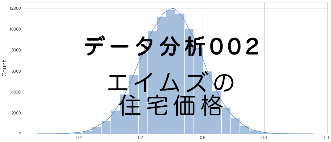
sns.histplot(df_test["SalePrice"],bins=20)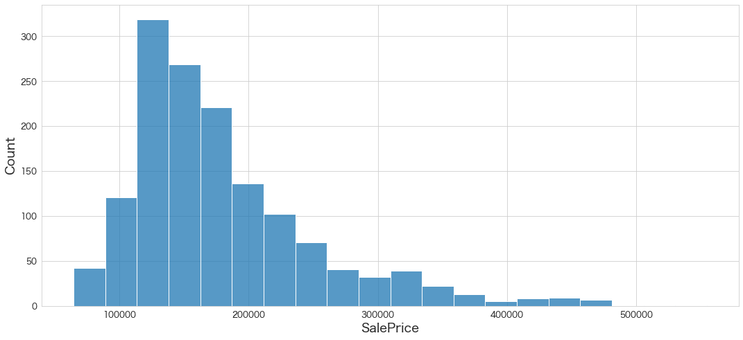
予測できていそうです。
Kaggleにスコア付与結果をアップロード
df_test[["Id","SalePrice"]].to_csv("ames_submission.csv",index=False)!/Users/hinomaruc/Desktop/blog/my-venv/bin/kaggle competitions submit -c house-prices-advanced-regression-techniques -f ames_submission.csv -m "#6 random forest bo"100%|██████████████████████████████████████| 33.7k/33.7k [00:03<00:00, 8.87kB/s] Successfully submitted to House Prices - Advanced Regression Techniques #6 random forest bo Score: 0.14587
デフォルトの設定より微妙に向上しました。
使用ライブラリのバージョン
pandas Version: 1.4.3
numpy Version: 1.22.4
scikit-learn Version: 1.1.1
seaborn Version: 0.11.2
matplotlib Version: 3.5.2
まとめ
ベイズ最適化(Bayesian Optimization)によるランダムフォーレストのパラメーターチューニングをしてみましたが、色々と関数を作り込むなど大変そうです。
パラメータは連続値しか試せませんでしたが、離散値や文字列なども対応しているか更なる調査は必要になりそうです。
次回は私が一番大好きなXGBoostを試してみたいと思います。
参考
・https://www.kdnuggets.com/2019/07/xgboost-random-forest-bayesian-optimisation.html