前回ARMAモデルの記事を書きました。

結果はARモデルやMAモデルと同じく1年分の日次予測は難しそうでした。
今回は自動ARIMAモデルを試してみます。
時系列モデル一覧
- AR (自己回帰モデル)
- MA (移動平均モデル)
- ARMA (自己回帰移動平均モデル)
- ARIMA (自己回帰和分移動平均モデル)
- ARIMAX (自己回帰和分移動平均モデル with 外因性変数)
- Auto ARIMA (自動ARIMAモデル)
- SARIMA (季節ARIMAモデル)
- SARIMAX (季節ARIMAモデル with 外因性変数)
- ARCH (分散自己回帰モデル)
- GARCH (一般化分散自己回帰モデル)
- VAR (ベクトル自己回帰モデル)
- VARMA (ベクトル自己回帰移動平均モデル)
※ ARIMAモデルについてはWikipedia参照
ARIMAモデルは、データが(…)平均に関して非定常性を示す場合に適用され、初期の差分ステップ(モデルの「Integrated 和分」部分に対応を1回以上適用して平均関数(すなわち、トレンド)の非定常性を排除することができる(...)。時系列に季節性が見られる場合は、季節成分を除去するために季節的差分を適用することができる
引用: https://ja.wikipedia.org/wiki/自己回帰和分移動平均モデル
ARIMAモデルは非定常過程を定常過程にするため差分ステップ(I)をARMAに取り入れより一般化したモデルのようです。
前回のARMAの記事でも、非定常過程を1階差分取ることによって定常過程へ変換しているので結果はほとんど同じになるかも知れません。
また今回は業務利用のことを考え、自動的にARIMAモデルを作成してくれるpmdarimaというライブラリを利用します。そのため、事前にpython3 -m pip install pmdarimaでライブラリをインストールしておきます。
- アップル引越しの引越し数をAuto-ARIMAモデルで予想する
- 本記事で利用したライブラリのバージョン
アップル引越しの引越し数をAuto-ARIMAモデルで予想する
モデル作成するパートまではARモデルと共通になります。
本記事では重複した内容になってしまうので、詳細な説明を省きます。
データの読み込み
# アップル引越しのデータセットを読み込む
import pandas as pd
from matplotlib import pyplot as plt
import pandas as pd
# 訓練データと予測付与用データの読み込み
df = pd.read_csv("/Users/hinomaruc/Desktop/blog/dataset/applehikkoshi/train.csv",parse_dates=['datetime'],index_col='datetime')
df_test = pd.read_csv("/Users/hinomaruc/Desktop/blog/dataset/applehikkoshi/test.csv",parse_dates=['datetime'],index_col='datetime')
# 描画設定
from IPython.display import HTML
import seaborn as sns
from matplotlib import ticker
import matplotlib.pyplot as plt
sns.set_style("whitegrid")
from matplotlib import rcParams
rcParams['font.family'] = 'Hiragino Sans' # Macの場合
#rcParams['font.family'] = 'Meiryo' # Windowsの場合
#rcParams['font.family'] = 'VL PGothic' # Linuxの場合
rcParams['xtick.labelsize'] = 12 # x軸のラベルのフォントサイズ
rcParams['ytick.labelsize'] = 12 # y軸のラベルのフォントサイズ
rcParams['axes.labelsize'] = 18 # ラベルのフォントとサイズ
rcParams['figure.figsize'] = 18,8 # 画像サイズの変更(inch)日付の間隔をasfreqメソッドで変更する
asfreqメソッドはpandasのメソッドで日付の粒度を変更してくれたり、足りない日付も作成してくれる便利なメソッドです。
# https://pandas.pydata.org/docs/reference/api/pandas.DataFrame.asfreq.html
# 日付の間隔を「日間隔」に変更 (元から日別のデータですが、、週や月間隔にも変更できます)
df = df.asfreq('d')df.info()DatetimeIndex: 2101 entries, 2010-07-01 to 2016-03-31 Freq: D Data columns (total 5 columns): # Column Non-Null Count Dtype --- ------ -------------- ----- 0 y 2101 non-null int64 1 client 2101 non-null int64 2 close 2101 non-null int64 3 price_am 2101 non-null int64 4 price_pm 2101 non-null int64 dtypes: int64(5) memory usage: 98.5 KB
欠損値の確認
df.infoメソッドで確認した通り、欠損値は今回存在しませんのでスキップします。
引っ越し数(y)を描画
pandasのplotメソッドで描画できます。
df.y.plot()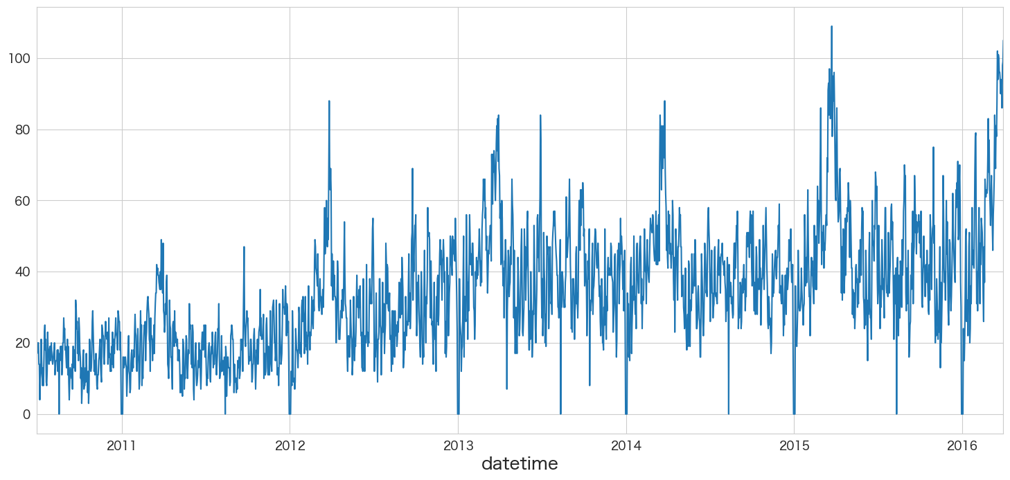
yが正規分布に従うかどうかQQプロットを確認
統計手法を適用するにあたり、おおよそ正規分布を仮定する必要があります。
そのためデータが正規分布に従っているかどうかQQプロットという手法を使って確認します。
# 正規分布に従うかどうかをQQプロットを描画して確認
import scipy.stats as stats
import matplotlib.pyplot as plt

plt.subplot(1,2,1)
sns.histplot(df["y"], kde=True)
plt.subplot(1,2,2)
stats.probplot(df["y"], dist="norm", plot=plt)
plt.show()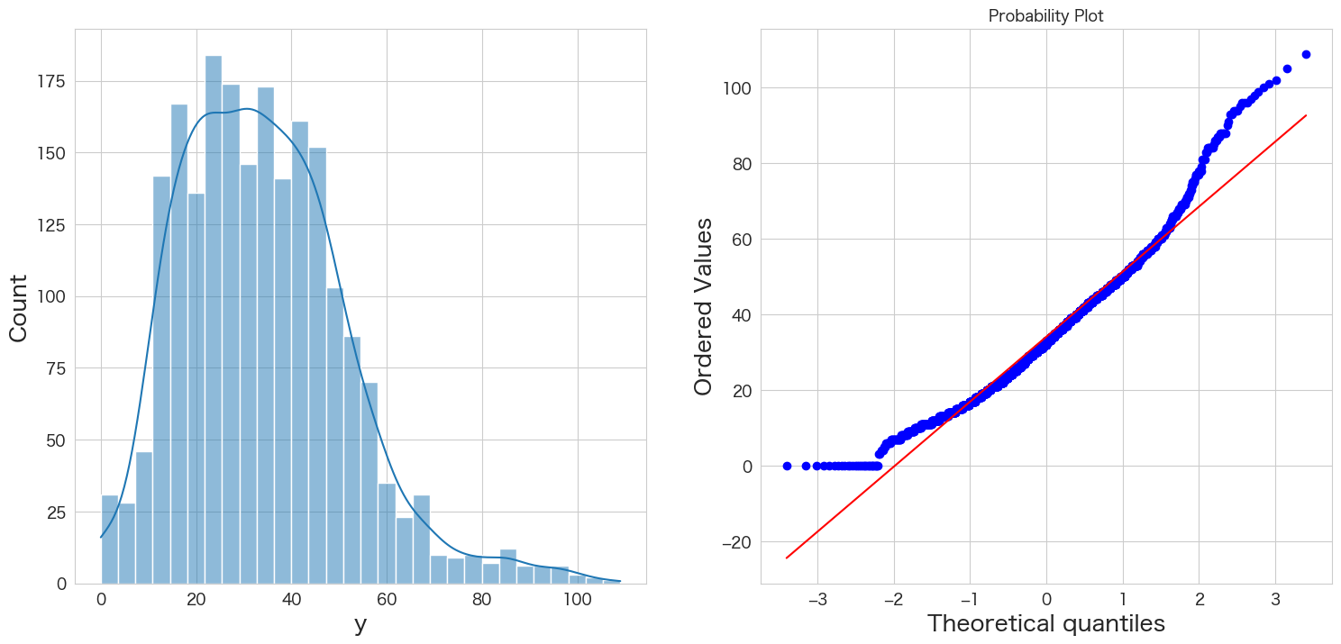
左側のグラフがヒストグラム、右側のグラフがQQプロットです。
青い点が赤い線に沿っていれば正規分布であるという表現方法になっています。
端の部分がずれているようですが、なんとなく正規分布に従っていると仮定します。
Mann-Kendall trend検定
H0: データにトレンドは存在しない
HA: データにトレンドが存在する
# https://pypi.org/project/pymannkendall/
import pymannkendall as mk
mk.original_test(df["y"])Mann_Kendall_Test(trend='increasing', h=True, p=0.0, z=30.51302505819748, Tau=0.4440819564379774, s=979667.0, var_s=1030826418.3333334, slope=0.016624040920716114, intercept=14.544757033248079)
p <= 0.05なので帰無仮説は棄却され、データにトレンドは存在するという結果になりました。
そのため、拡張ディッキー・フラー検定ではトレンドがあるということを示すregression='ct'のオプションを追加しようと思います。
拡張ディッキー・フラー検定で時系列データが(弱)定常か非定常か確認する
帰無仮説と対立仮説は下記になります。
H0: 単位根がある
HA: 単位根がない
# https://www.statsmodels.org/dev/generated/statsmodels.tsa.stattools.adfuller.html
from statsmodels.tsa.stattools import adfuller

# 検定結果を見やすく加工
result = adfuller(df["y"],regression='ct')
labels = ["検定統計量","P値","#ラグ数","#観測数"]
mod_result = pd.Series(result[0:4],index=labels)
for key,val in result[4].items():
    mod_result[f'臨界値 (有意水準:{key})'] = val;
mod_result検定統計量 -3.139726 P値 0.097095 #ラグ数 26.000000 #観測数 2074.000000 臨界値 (有意水準:1%) -3.963142 臨界値 (有意水準:5%) -3.412609 臨界値 (有意水準:10%) -3.128298 dtype: float64
P値が0.05以下ではないため帰無仮説を棄却できず「単位根がないとは言えない」という結果になります。
つまりアップル引っ越しのデータセットは弱定常過程ではなく、非定常過程の可能性がありそうです。
非定常過程のデータを定常過程のデータに変換する (階差)
ARIMAモデルは「I」ntegratedの部分で差分を取るようなので今回このパートはスキップします。
ARIMAモデルの作成
自動ARIMAモデルを実行する前に単純なARIMA(1,1,1)のモデル△yt=c+ϕ1△yt-1 +θ1εt-1+εtを作成していこうと思います。
式の中身を分解すると下記になります。
・cはコンスタント値
・△ytは現在の値と1ピリオド前の値の差分
・△yt-1は1ピリオド前の値の2ピリオド前の値の差分
・εtは現在の残差(エラー)
・εt-1は1ピリオド前の残差(エラー)
・ϕは現在値を説明するのに過去の値がどれほど関連しているか (ARの部分)
・θは現在値を説明するのに過去の残差(エラー)がどれほど関連しているか (MAの部分)
ARモデルとMAモデルは対数尤度比検定(Log likelihood ratio test)でモデルん優劣を判断していましたが、簡略化のため、log likelihooodの値とAICの値を判断材料にしようと思います。log likelihooodの値は高いほどいいモデル、AICの値は低いほどいいモデルという判別になります。
それではARIMAモデルの作成をしていきたいと思います。
from statsmodels.tsa.arima.model import ARIMA
# ARIMA(1,1,1)モデルの作成
ar1i1ma1_model = ARIMA(df.y,order=(1,1,1))
ar1i1ma1_model_fit = ar1i1ma1_model.fit()
ar1i1ma1_model_fit.summary()
SARIMAX Results

  Dep. Variable:           y          No. Observations:     2101


  Model:            ARIMA(1, 1, 1)    Log Likelihood      -7537.008


  Date:            Thu, 22 Sep 2022   AIC                 15080.017


  Time:                15:06:34       BIC                 15096.966


  Sample:             07-01-2010      HQIC                15086.225


                     - 03-31-2016


  Covariance Type:        opg


            coef     std err      z      P>|z|  [0.025    0.975]


  ar.L1      0.6371     0.020    31.144  0.000     0.597     0.677


  ma.L1     -0.9273     0.011   -86.794  0.000    -0.948    -0.906


  sigma2    76.6991     1.785    42.962  0.000    73.200    80.198


  Ljung-Box (L1) (Q):     0.28   Jarque-Bera (JB):   217.41


  Prob(Q):                0.59   Prob(JB):            0.00


  Heteroskedasticity (H): 2.53   Skew:                -0.08


  Prob(H) (two-sided):    0.00   Kurtosis:            4.57


Warnings:
[1] Covariance matrix calculated using the outer product of gradients (complex-step).
arima(1,1,1)ではconstantが出力されないようですね。
For example, a constant cannot be included in an ARIMA(1, 1, 1) modelと書いてあるので、d > 0なのが関係あるのかもしれません。
ValueError: In models with integration (
d > 0) or seasonal integration (D > 0), trend terms of lower order thand + Dcannot be (as they would be eliminated due to the differencing operation). For example, a constant cannot be included in an ARIMA(1, 1, 1) model, but including a linear trend, which would have the same effect as fitting a constant to the differenced data, is allowed. 引用: statsmodelsのソース
pmdarimaで自動ARIMAモデルを作成する
import numpy as np
import pmdarima as pm

# http://alkaline-ml.com/pmdarima/modules/generated/pmdarima.arima.AutoARIMA.html
stepwise_fit = pm.auto_arima(df.y, start_p=5, start_q=5,max_p=50, max_q=50,
                                            trace=True,
                                            suppress_warnings=True,  # warningsを出さないようにする
                                            stepwise=True # stepwiseでやる
) Performing stepwise search to minimize aic ARIMA(5,1,5)(0,0,0)[0] intercept : AIC=14763.179, Time=7.69 sec ARIMA(0,1,0)(0,0,0)[0] intercept : AIC=15355.426, Time=0.07 sec ARIMA(1,1,0)(0,0,0)[0] intercept : AIC=15280.829, Time=0.12 sec ARIMA(0,1,1)(0,0,0)[0] intercept : AIC=15251.602, Time=0.36 sec ARIMA(0,1,0)(0,0,0)[0] : AIC=15353.468, Time=0.08 sec ARIMA(4,1,5)(0,0,0)[0] intercept : AIC=inf, Time=8.17 sec ARIMA(5,1,4)(0,0,0)[0] intercept : AIC=14788.005, Time=5.15 sec ARIMA(6,1,5)(0,0,0)[0] intercept : AIC=inf, Time=8.13 sec ARIMA(5,1,6)(0,0,0)[0] intercept : AIC=14777.352, Time=6.95 sec ARIMA(4,1,4)(0,0,0)[0] intercept : AIC=inf, Time=5.73 sec ARIMA(4,1,6)(0,0,0)[0] intercept : AIC=inf, Time=7.95 sec ARIMA(6,1,4)(0,0,0)[0] intercept : AIC=14771.147, Time=8.57 sec ARIMA(6,1,6)(0,0,0)[0] intercept : AIC=inf, Time=9.52 sec ARIMA(5,1,5)(0,0,0)[0] : AIC=14762.157, Time=3.19 sec ARIMA(4,1,5)(0,0,0)[0] : AIC=inf, Time=4.75 sec ARIMA(5,1,4)(0,0,0)[0] : AIC=inf, Time=2.90 sec ARIMA(6,1,5)(0,0,0)[0] : AIC=inf, Time=5.74 sec ARIMA(5,1,6)(0,0,0)[0] : AIC=inf, Time=4.24 sec ARIMA(4,1,4)(0,0,0)[0] : AIC=inf, Time=2.93 sec ARIMA(4,1,6)(0,0,0)[0] : AIC=inf, Time=5.15 sec ARIMA(6,1,4)(0,0,0)[0] : AIC=14769.149, Time=3.90 sec ARIMA(6,1,6)(0,0,0)[0] : AIC=inf, Time=5.41 sec Best model: ARIMA(5,1,5)(0,0,0)[0] Total fit time: 106.732 seconds
ARIMA(5,1,5)(0,0,0)[0]が選択されました。
2分経たないうちに結果が返ってきました。stepwiseの効果でしょうか、とても早いです。
# ベストモデルのサマリ情報の確認
stepwise_fit.summary()
SARIMAX Results

  Dep. Variable:           y          No. Observations:     2101


  Model:           SARIMAX(5, 1, 5)   Log Likelihood      -7370.078


  Date:            Thu, 22 Sep 2022   AIC                 14762.157


  Time:                17:16:10       BIC                 14824.303


  Sample:             07-01-2010      HQIC                14784.919


                     - 03-31-2016


  Covariance Type:        opg


            coef     std err      z      P>|z|  [0.025    0.975]


  ar.L1      1.0450     0.061    17.016  0.000     0.925     1.165


  ar.L2     -1.5852     0.054   -29.507  0.000    -1.691    -1.480


  ar.L3      1.0748     0.081    13.264  0.000     0.916     1.234


  ar.L4     -1.1188     0.043   -26.040  0.000    -1.203    -1.035


  ar.L5      0.2284     0.051     4.441  0.000     0.128     0.329


  ma.L1     -1.3958     0.057   -24.468  0.000    -1.508    -1.284


  ma.L2      1.8550     0.067    27.758  0.000     1.724     1.986


  ma.L3     -1.5318     0.086   -17.863  0.000    -1.700    -1.364


  ma.L4      1.2891     0.054    23.956  0.000     1.184     1.395


  ma.L5     -0.5048     0.041   -12.352  0.000    -0.585    -0.425


  sigma2    63.4711     1.480    42.898  0.000    60.571    66.371


  Ljung-Box (L1) (Q):     1.24   Jarque-Bera (JB):   234.83


  Prob(Q):                0.27   Prob(JB):            0.00


  Heteroskedasticity (H): 2.36   Skew:                -0.19


  Prob(H) (two-sided):    0.00   Kurtosis:            4.60


Warnings:
[1] Covariance matrix calculated using the outer product of gradients (complex-step).
ar.L1~ ar.L5もma.L1 ~ ma.L5もP>|z| が0.05以下なので意味がある係数ということになり問題なさそうです。
(オプション) 残差の最適な数値を求める
ARIMAモデルの「I」の部分の値を求めます。
auto-ARIMAで自動的に求めてくれるようですが、明示的に値をオプションに指定してあげることによって処理が効率化されるようです。
下記にサンプルがあるので、そのまま利用します。

from pmdarima.arima import ndiffs

kpss_diffs = ndiffs(df.y, alpha=0.05, test='kpss', max_d=10)
adf_diffs = ndiffs(df.y, alpha=0.05, test='adf', max_d=10)
n_diffs = max(adf_diffs, kpss_diffs)

print(f"Estimated differencing term: {n_diffs}")Estimated differencing term: 1
ARIMAの「I」は1が良さそうという結果になりました。
ARMAモデル作成する前も何階差とるべきかこの方法で求めてあげるべきでしたね。
作成したARIMAモデルの残差分析
残差の正規性はQQプロットで確認することにします。残差の間に相関がない(独立している)ことはLjung-Box検定で確認します。
resid = stepwise_fit.resid()
# ARIMA(5,1,5)の残差データを確認
resid.plot()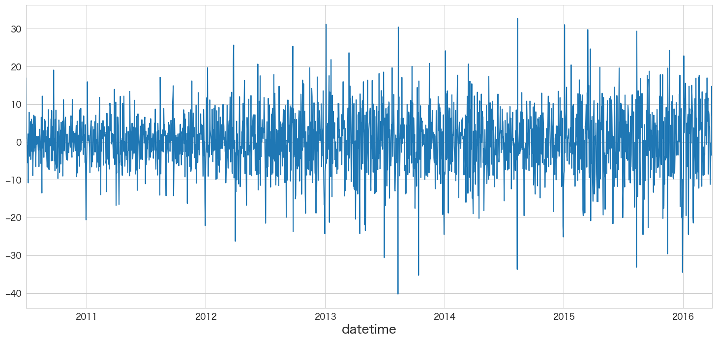
残差の平均と分散を確認
print(f"mean:{resid.mean()}、variance:{resid.var()}")mean:0.08623452413743744、variance:65.49448487344031
残差の正規性の確認
# 正規分布に従うかどうかをQQプロットを描画して確認
import scipy.stats as stats
import matplotlib.pyplot as plt

plt.subplot(1,2,1)
sns.histplot(resid, kde=True)
plt.subplot(1,2,2)
stats.probplot(resid, dist="norm", plot=plt)
plt.show()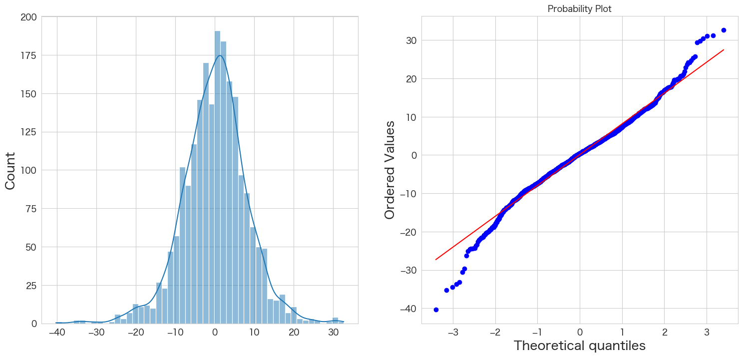
概ね正規分布に従っていそうです。
自己相関係数の確認
# 自己相関係数の確認
import pandas as pd
import matplotlib.pyplot as plt
from statsmodels.graphics.tsaplots import plot_acf
import numpy as np

fig, ax = plt.subplots(figsize=(16,8))
plot_acf(resid, lags=50, zero=False, title="自己相関係数 (autocorrelation)", ax=ax, alpha=0.01)
plt.ylim([0,1])
plt.yticks(np.arange(0.1, 1.1, 0.1))
plt.xticks(np.arange(1, 51, 1))
plt.show()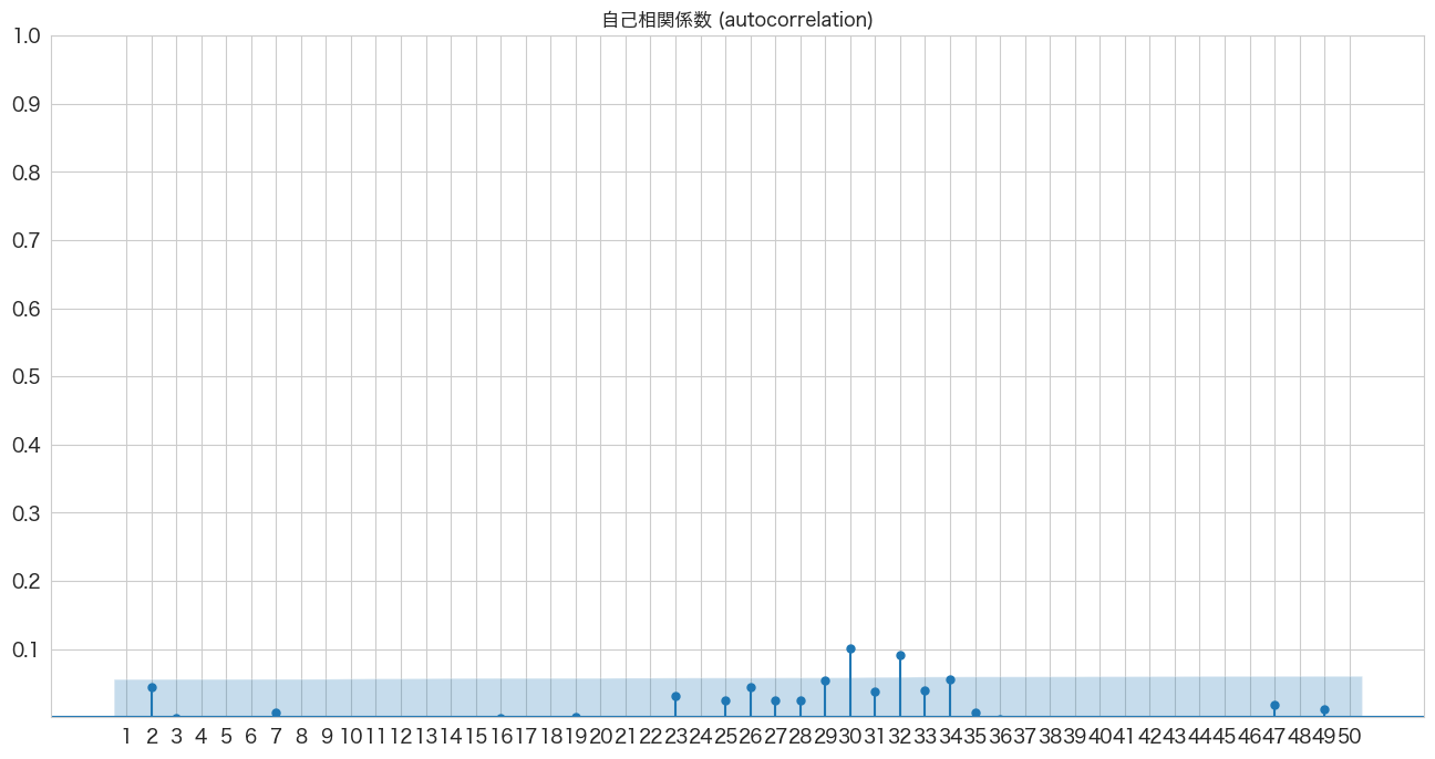
若干青いエリアから外れていますが概ね問題なさそうです。
Ljung-Box検定で残差の独立性の確認
H0: 残差は独立分布している
HA: 残差は独立分布ではない
残差が独立分布していることが望ましいので帰無仮説を棄却しない(P値 >= 0.05)結果になることを期待したいと思います。
# https://www.statsmodels.org/stable/generated/statsmodels.stats.diagnostic.acorr_ljungbox.html

import statsmodels.api as sm
sm.stats.acorr_ljungbox(resid,lags=10)
lb_stat lb_pvalue 1 1.224429 0.268493 2 5.256696 0.072198 3 5.257660 0.153873 4 5.795151 0.214978 5 6.502117 0.260378 6 8.206492 0.223362 7 8.315527 0.305595 8 11.403611 0.179862 9 25.530109 0.002437 10 36.186839 0.000078
1~10のラグで検定してみました。ラグ9とラグ10以外の全てのp値が0.05以上なので問題ないということにします。
残差分析の結果
残差分析の結果は、ARIMA(5,1,5)の残差が平均0の正規分布に従い、一応ラグ8まで残差の間には相関がないので問題ないということにします。
ARIMA(5,1,5)モデルを使って引っ越し数を予測する
そんなにARMAモデルから変化がないかも知れませんがやってみます。
# 2016-04-01 ~ 2017-03-31までの階差を予測
stepwise_fit.predict(n_periods=365,X=df_test.index).plot()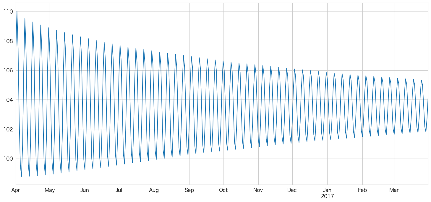
# 学習データの引っ越し数の値(青い線)と予測した引っ越し数の値(オレンジの線)を描画
plt.figure(figsize=(20, 3))

ytrue = df.y.iloc[-31:]
ypred = stepwise_fit.predict(n_periods=365,X=df_test.index)

plt.plot(ytrue, label="Training Data")
plt.plot(ypred, label="Forecasts")

plt.title("apple-hikkoshi prediction")
_ = plt.legend()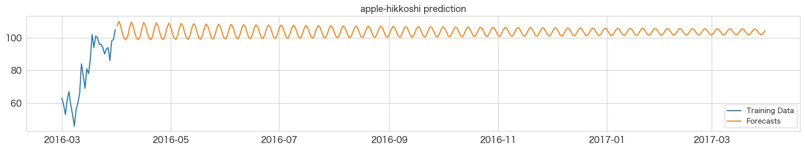
結果は対して変わらずでした。。
まとめ
pmdarimaライブラリはstatsmodels.tsa.arima.model.ARIMAとほぼ同じ使い方でアウトプットフォーマットもそっくりです。
使うならより機能が豊富なpmdarima一択かなと思います。
ARIMAモデルでも1年分の日別予測は難しかったので、次は季節性を考慮したSARIMAモデルを試します。
SARIMAモデルもpmdarimaで構築可能なので似たようなコードになると思います。
本記事で利用したライブラリのバージョン
import pandas as pd
import numpy as np
import statsmodels as sm
import matplotlib as mpl
import pymannkendall as mk
import scipy as scp
print('pandas',pd.__version__)
print('numpy',np.__version__)
print('statsmodels',sm.__version__)
print('matplotlib',mpl.__version__)
print('pymannkendall',mk.__version__)
print('scipy',scp.__version__)pandas 1.4.3 numpy 1.23.2 statsmodels 0.13.2 matplotlib 3.5.3 pymannkendall 1.4.2 scipy 1.9.1