今回からアップル引越しのデータを使って時系列予測モデルを作成していきます。
最初からAutoMLであるAutoGluonを使ってしまうと思っています。
サンプルデータを使って動作確認をした記事もありますので補足情報にお使いください。
GPU環境の情報を確認
# CUDAのバージョンの確認
!nvcc --versionnvcc: NVIDIA (R) Cuda compiler driver Copyright (c) 2005-2020 NVIDIA Corporation Built on Mon_Oct_12_20:09:46_PDT_2020 Cuda compilation tools, release 11.1, V11.1.105 Build cuda_11.1.TC455_06.29190527_0
cudaのバージョンは11.1のようです。
# インストール済みのcudaのバージョンを確認
!ls -la /usr/local/ | grep cudalrwxrwxrwx 1 root root 22 Aug 15 13:37 cuda -> /etc/alternatives/cuda drwxr-xr-x 16 root root 4096 Aug 15 13:29 cuda-10.0 drwxr-xr-x 15 root root 4096 Aug 15 13:31 cuda-10.1 lrwxrwxrwx 1 root root 25 Aug 15 13:37 cuda-11 -> /etc/alternatives/cuda-11 drwxr-xr-x 15 root root 4096 Aug 15 13:34 cuda-11.0 drwxr-xr-x 1 root root 4096 Aug 15 13:36 cuda-11.1
CUDA10.0、10.1、11.0、11.1がインストール済みで利用可能のようです。
# GPU関連の情報を表示
!nvidia-smiMon Aug 22 12:54:14 2022 +-----------------------------------------------------------------------------+ | NVIDIA-SMI 460.32.03 Driver Version: 460.32.03 CUDA Version: 11.2 | |-------------------------------+----------------------+----------------------+ | GPU Name Persistence-M| Bus-Id Disp.A | Volatile Uncorr. ECC | | Fan Temp Perf Pwr:Usage/Cap| Memory-Usage | GPU-Util Compute M. | | | | MIG M. | |===============================+======================+======================| | 0 Tesla T4 Off | 00000000:00:04.0 Off | 0 | | N/A 72C P0 33W / 70W | 2556MiB / 15109MiB | 0% Default | | | | N/A | +-------------------------------+----------------------+----------------------+ +-----------------------------------------------------------------------------+ | Processes: | | GPU GI CI PID Type Process name GPU Memory | | ID ID Usage | |=============================================================================| +-----------------------------------------------------------------------------+
Driver Version: 460.32.03、GPUはTesla T4が割当られているようです。
AutoGluonのインストール
https://auto.gluon.ai/stable/install.html を参考にインストールしていきます。
ちなみに今回はLinux、PIP、GPUでのインストール手順を選択しています。
# torchがインストールしてあるかどうか確認
!pip freeze | grep torchtorch @ https://download.pytorch.org/whl/cu113/torch-1.12.1%2Bcu113-cp37-cp37m-linux_x86_64.whl torchaudio @ https://download.pytorch.org/whl/cu113/torchaudio-0.12.1%2Bcu113-cp37-cp37m-linux_x86_64.whl torchsummary==1.5.1 torchtext==0.13.1 torchvision @ https://download.pytorch.org/whl/cu113/torchvision-0.13.1%2Bcu113-cp37-cp37m-linux_x86_64.whl
たまたまかも知れませんが、22年8月現在ColabではAutoGluonの使用でダウンロードすべきcu113のtorchがインストールされているようです。ただし、torchのバージョンが1.12.1のようです。(公式サイトでは、1.21.0-cu113をインストールするようになっている。)
# mxnetがインストールしてあるかどうか確認
!pip freeze | grep mxnet結果なし
mxnetはインストールされていませんでした。
CUDA10.1はインストール済みだったので、mxnetライブラリはmxnet-cu101のバージョンをインストールすれば問題なさそうです。
torchもAutoGluonの公式サイトではtorch-1.12.0+cu113をインストールするようになっていましたが、マイナーバージョンが少し異なるだけなのでこのままAutoGluonのインストール作業を進めていきます。
# mxnet-cu101のインストール
!python3 -m pip install "mxnet_cu101<2.0.0, >=1.7.0"
Looking in indexes: https://pypi.org/simple, https://us-python.pkg.dev/colab-wheels/public/simple/
Collecting mxnet_cu101<2.0.0,>=1.7.0
  Downloading mxnet_cu101-1.9.1-py3-none-manylinux2014_x86_64.whl (360.0 MB)
     |████████████████████████████████| 360.0 MB 18 kB/s
Requirement already satisfied: requests<3,>=2.20.0 in /usr/local/lib/python3.7/dist-packages (from mxnet_cu101<2.0.0,>=1.7.0) (2.23.0)
Collecting graphviz<0.9.0,>=0.8.1
  Downloading graphviz-0.8.4-py2.py3-none-any.whl (16 kB)
Requirement already satisfied: numpy<2.0.0,>1.16.0 in /usr/local/lib/python3.7/dist-packages (from mxnet_cu101<2.0.0,>=1.7.0) (1.21.6)
Requirement already satisfied: urllib3!=1.25.0,!=1.25.1,<1.26,>=1.21.1 in /usr/local/lib/python3.7/dist-packages (from requests<3,>=2.20.0->mxnet_cu101<2.0.0,>=1.7.0) (1.24.3)
Requirement already satisfied: idna<3,>=2.5 in /usr/local/lib/python3.7/dist-packages (from requests<3,>=2.20.0->mxnet_cu101<2.0.0,>=1.7.0) (2.10)
Requirement already satisfied: certifi>=2017.4.17 in /usr/local/lib/python3.7/dist-packages (from requests<3,>=2.20.0->mxnet_cu101<2.0.0,>=1.7.0) (2022.6.15)
Requirement already satisfied: chardet<4,>=3.0.2 in /usr/local/lib/python3.7/dist-packages (from requests<3,>=2.20.0->mxnet_cu101<2.0.0,>=1.7.0) (3.0.4)
Installing collected packages: graphviz, mxnet-cu101
  Attempting uninstall: graphviz
    Found existing installation: graphviz 0.10.1
    Uninstalling graphviz-0.10.1:
      Successfully uninstalled graphviz-0.10.1
Successfully installed graphviz-0.8.4 mxnet-cu101-1.9.1
mxnet_cu101-1.9.1がインストールされました。
# ColabでインストールされているgymがAutoGluonインストール時にincompatible*1になるので、削除
# (*1 gym 0.17.3 requires cloudpickle<1.7.0,>=1.2.0)
!pip uninstall gym -y

# autogluonのインストール (22年8月現在の最新版)
!pip install autogluon==0.5.2Found existing installation: gym 0.25.1 Uninstalling gym-0.25.1: Successfully uninstalled gym-0.25.1 Looking in indexes: https://pypi.org/simple, https://us-python.pkg.dev/colab-wheels/public/simple/ Collecting autogluon==0.5.2 Downloading autogluon-0.5.2-py3-none-any.whl (9.6 kB) ・・・省略・・・ Successfully installed Pillow-9.0.1 antlr4-python3-runtime-4.8 autocfg-0.0.8 autogluon-0.5.2 autogluon-contrib-nlp-0.0.1b20220208 autogluon.common-0.5.2 autogluon.core-0.5.2 autogluon.features-0.5.2 autogluon.multimodal-0.5.2 autogluon.tabular-0.5.2 autogluon.text-0.5.2 autogluon.timeseries-0.5.2 autogluon.vision-0.5.2 boto3-1.24.56 botocore-1.27.56 catboost-1.0.6 colorama-0.4.5 contextvars-2.4 dask-2021.11.2 deprecated-1.2.13 distlib-0.3.5 distributed-2021.11.2 fairscale-0.4.6 flake8-3.9.2 gluoncv-0.10.5.post0 gluonts-0.9.8 grpcio-1.43.0 huggingface-hub-0.8.1 hyperopt-0.2.7 immutables-0.18 jmespath-1.0.1 lightgbm-3.3.2 mccabe-0.6.1 nlpaug-1.1.10 nptyping-1.4.4 omegaconf-2.1.2 platformdirs-2.5.2 pmdarima-1.8.5 portalocker-2.5.1 psutil-5.8.0 py4j-0.10.9.7 pyDeprecate-0.3.2 pycodestyle-2.7.0 pyflakes-2.3.1 pytorch-lightning-1.6.5 pytorch-metric-learning-1.3.2 ray-1.13.0 s3transfer-0.6.0 sacrebleu-2.2.0 sacremoses-0.0.53 scikit-image-0.19.3 sentencepiece-0.1.95 sktime-0.11.4 tbats-1.1.0 tensorboardX-2.5.1 timm-0.5.4 tokenizers-0.12.1 torchmetrics-0.7.3 transformers-4.20.1 typish-1.9.3 urllib3-1.25.11 virtualenv-20.16.3 xgboost-1.4.2 yacs-0.1.8
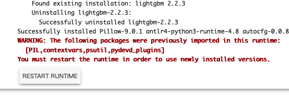
WARNING: The following packages were previously imported in this runtime:
[PIL,contextvars,psutil,pydevd_plugins,urllib3,yaml]
You must restart the runtime in order to use newly installed versions.
とWARNINGが出るので、RESTART RUNTIMEボタンを押して再起動します。
図:RESTART RUNTIMEボタン
# autogluonがインストールされているか確認
!pip freeze | grep autogluonautogluon==0.5.2 autogluon-contrib-nlp==0.0.1b20220208 autogluon.common==0.5.2 autogluon.core==0.5.2 autogluon.features==0.5.2 autogluon.multimodal==0.5.2 autogluon.tabular==0.5.2 autogluon.text==0.5.2 autogluon.timeseries==0.5.2 autogluon.vision==0.5.2
RUNTIMEを再起動してもインストールされたままでした。よかった。
AutoGluonでアップル引越しの時系列予測をやってみる
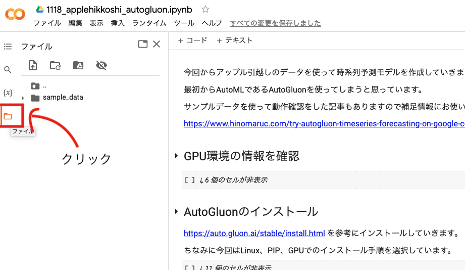
train.csvとtest.csvをColab環境にアップロード
-
左側のパネルのフォルダアイコンをクリック
-
データセットをドラッグ&ドロップします
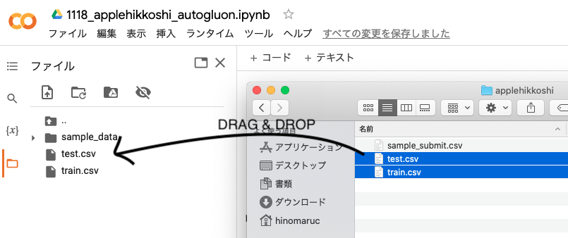
-
OKを押します

これでカレントディレクトリ(/content以下)にデータを配置出来たので、アクセス可能になります。
データの読み込み
# アップル引越しのデータセットを読み込む
import pandas as pd
from matplotlib import pyplot as plt
from autogluon.timeseries import TimeSeriesPredictor, TimeSeriesDataFrame
df = pd.read_csv("train.csv" , parse_dates=["datetime"], dtype={'y':'float64'})
df_test = pd.read_csv("test.csv" , parse_dates=["datetime"], dtype={'y':'float64'})
目的変数はfloat64でないとAutoETSやARIMAモデル作成時にエラーになってしまったので変換しました。
モデル作成時に下記のようなエラーが出たらfloat64に変換してみてください。
Buffer dtype mismatch, expected 'float64_t' but got 'long'
# データフレームの概要を確認
df.info()RangeIndex: 2101 entries, 0 to 2100 Data columns (total 6 columns): # Column Non-Null Count Dtype --- ------ -------------- ----- 0 datetime 2101 non-null datetime64[ns] 1 y 2101 non-null float64 2 client 2101 non-null int64 3 close 2101 non-null int64 4 price_am 2101 non-null int64 5 price_pm 2101 non-null int64 dtypes: datetime64[ns](1), float64(1), int64(4) memory usage: 98.6 KB
DataFrameをTimeSeriesDataFrameに変換する
# DataFrameをTimeSeriesDataFrameに変換する時にitem_idというカラムが必要
# item_idはデータのグループを指す。今回はグループは存在しないので一律同じ値を入力した。
df["item_id"] = 0
df.head()
datetime y client close price_am price_pm item_id 0 2010-07-01 17.0 0 0 -1 -1 0 1 2010-07-02 18.0 0 0 -1 -1 0 2 2010-07-03 20.0 0 0 -1 -1 0 3 2010-07-04 20.0 0 0 -1 -1 0 4 2010-07-05 14.0 0 0 -1 -1 0
# https://auto.gluon.ai/stable/api/autogluon.predictor.html#timeseriesdataframe
# データフレームをTimeSeriesDataFrame型に変換
train_data = TimeSeriesDataFrame.from_data_frame(df,timestamp_column="datetime")
# TimeSeriesDataFrameに変換したデータを確認
train_data.head()
y client close price_am price_pm item_id timestamp 0 2010-07-01 17.0 0 0 -1 -1 2010-07-02 18.0 0 0 -1 -1 2010-07-03 20.0 0 0 -1 -1 2010-07-04 20.0 0 0 -1 -1 2010-07-05 14.0 0 0 -1 -1
まずはお試しで31日間の予測をしどれくらいの精度になりそうか確認してみる
# 予測期間 (今回のケースだと31日間)
prediction_length = 31

# メソッドの中身ではdeep copyになっている
test_data = train_data.copy()

# 2016年3月をテスト用、それ以外を学習用データにする
train_data = train_data.slice_by_timestep(slice(None, -prediction_length))
plt.figure(figsize=(20, 3))
plt.plot(test_data.loc[0]["y"], label="test")
plt.plot(train_data.loc[0]["y"], label="train")
# テスト期間を強調する
plt.fill_betweenx(
y=(0, test_data.loc[0]["y"].max()),
x1=test_data.loc[0].index.max(),
x2=train_data.loc[0].index.max(),
alpha=0.1,
label="test interval",
)
plt.legend()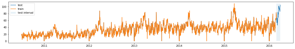
オレンジ色が学習期間、青色が予測期間になります。
!rm -rf autogluon-applehikkoshi
# https://auto.gluon.ai/stable/api/autogluon.predictor.html#module-5

# 予測モデルの設定
predictor = TimeSeriesPredictor(
    path="autogluon-applehikkoshi",
    target="y", # 目的変数
    prediction_length=prediction_length,
    eval_metric="RMSE"
)

# 学習する
predictor.fit(train_data=train_data,presets="medium_quality")
INFO:autogluon.timeseries.predictor:presets is set to medium_quality
INFO:autogluon.timeseries.predictor:================ TimeSeriesPredictor ================
INFO:autogluon.timeseries.predictor:TimeSeriesPredictor.fit() called
INFO:autogluon.timeseries.predictor:Setting presets to: medium_quality
INFO:autogluon.timeseries.predictor:Fitting with arguments:
INFO:autogluon.timeseries.predictor:{'evaluation_metric': 'RMSE',
 'hyperparameter_tune_kwargs': None,
 'hyperparameters': 'default',
 'prediction_length': 31,
 'target_column': 'y',
 'time_limit': None}
INFO:autogluon.timeseries.predictor:Provided training data set with 2070 rows, 1 items. Average time series length is 2070.0.
INFO:autogluon.timeseries.predictor:Training artifacts will be saved to: /content/autogluon-applehikkoshi
・・・省略・・・
INFO:autogluon.timeseries.trainer:Training complete. Models trained: ['AutoETS', 'ARIMA', 'SimpleFeedForward', 'DeepAR', 'Transformer', 'WeightedEnsemble']
INFO:autogluon.timeseries.trainer:Total runtime: 732.48 s
INFO:autogluon.timeseries.trainer:Best model: WeightedEnsemble
INFO:autogluon.timeseries.trainer:Best model score: -8.7507
だいたい15分ほどで完了しました。DeepARで時間がかかりました。WeightedEnsembleが選ばれました。
# 作成モデルの一覧を表示する
predictor.leaderboard(test_data, silent=True)
model score_test score_val pred_time_test pred_time_val fit_time_marginal fit_order 0 Transformer -7.172322 -10.433371 0.367382 0.344499 196.790241 5 1 WeightedEnsemble -8.838028 -8.750748 2.526231 1.003680 1.280201 6 2 DeepAR -9.573973 -9.724971 0.470696 0.457473 417.433229 4 3 AutoETS -17.875232 -18.634539 0.852930 0.109731 0.241552 1 4 SimpleFeedForward -18.736877 -11.294595 0.032008 0.021253 113.388606 3 5 ARIMA -28.201587 -17.012414 1.105978 0.180454 1.003976 2
score_valの値が一番良かったのがWeightedEnsembleなので、選択されたようです。次点でDeepARが精度が良かったようです。
WeightedEnsembleなので、fit_orderが1~5番のモデルを重みを変えて組み合わせた結果でしょうか?
# ベストモデル
predictor.get_model_best() 'WeightedEnsemble'
# 予測データ作成
predictions = predictor.predict(train_data,"WeightedEnsemble")
# 2016年3月の予測結果
predictions.loc[0]
mean 0.1 0.2 0.3 0.4 0.5 0.6 0.7 0.8 0.9 timestamp 2016-03-01 60.607901 48.610853 52.512298 56.704144 59.470130 61.284553 62.844764 64.971739 67.668370 72.020470 2016-03-02 57.338657 45.876428 50.460668 52.735242 54.506025 56.365934 58.461636 61.862424 65.268460 69.144131 2016-03-03 56.421616 44.447008 49.058497 51.723610 53.952413 56.169531 58.341299 61.107270 64.033074 68.715897 2016-03-04 59.315572 49.095956 52.421152 55.101598 57.319467 59.378345 60.971272 63.323452 66.194820 70.193901 2016-03-05 60.984202 49.334495 53.224692 56.052357 58.211470 60.152153 62.605994 65.038977 68.738808 74.420179 2016-03-06 60.154552 47.955532 51.980402 54.888346 57.729883 60.067365 62.153181 65.101131 68.626732 72.986518 2016-03-07 55.997976 43.944043 47.862171 51.170888 53.800930 55.597699 57.536124 60.668880 63.654367 69.579834 2016-03-08 55.715753 42.443749 46.680211 50.551846 52.905301 54.975713 57.520776 60.697680 63.964450 70.137777 2016-03-09 56.814999 42.057283 47.641024 51.959750 54.461087 57.006904 59.431330 62.688595 65.467281 70.736449 2016-03-10 59.193336 45.295066 50.043875 53.720311 56.499875 59.208808 61.318894 64.487754 68.450824 73.334892 2016-03-11 67.525128 53.570807 58.653490 61.433828 64.837652 67.208084 69.260971 72.372408 77.709054 81.431354 2016-03-12 72.332047 57.218694 61.809976 65.811335 69.060285 72.142821 75.707870 78.160344 82.552576 88.681445 2016-03-13 74.895305 56.483266 62.012808 67.164286 70.215048 75.512518 79.189081 82.262850 86.953144 94.480359 2016-03-14 78.411033 60.412886 66.346583 72.174657 75.552630 78.590703 81.474543 84.690336 89.569188 95.798509 2016-03-15 79.326524 61.907382 68.173013 72.299028 75.774260 79.153304 82.175620 85.456185 90.114237 96.374174 2016-03-16 84.470267 65.773581 73.277789 77.682233 81.593586 84.479475 87.448114 91.477794 95.347348 102.369241 2016-03-17 87.075908 69.858175 76.721585 80.126436 83.743251 86.561700 90.507810 93.857730 97.878571 104.926400 2016-03-18 88.818798 72.159138 77.375337 81.848732 85.571174 88.806468 91.472654 95.344882 99.527021 107.087340 2016-03-19 89.961329 71.222729 78.422071 82.860429 85.939257 90.729468 93.580227 98.757196 102.051305 107.250524 2016-03-20 92.342297 71.873437 79.809660 83.851805 87.172088 90.991120 95.072043 100.209838 105.102294 114.697367 2016-03-21 91.727498 72.578070 79.158758 83.214814 87.299721 91.797659 96.685995 99.895382 104.278673 109.985152 2016-03-22 92.060761 69.018830 77.263642 83.535674 88.107313 92.977502 96.638539 99.512526 106.474702 113.956245 2016-03-23 90.533393 70.748470 78.703196 83.601522 87.577676 91.144138 93.927504 97.582536 102.705020 108.583368 2016-03-24 90.608582 71.520009 78.370797 82.218972 86.213341 89.439376 92.231554 97.495874 103.266502 111.511284 2016-03-25 87.188481 66.027736 73.390742 78.852372 83.406344 87.706514 90.716616 95.436747 99.768813 108.224185 2016-03-26 86.539641 65.166218 73.306287 77.877481 82.878745 86.161068 89.763110 94.353225 100.338912 107.391733 2016-03-27 82.330292 60.627883 66.742187 73.619625 78.231057 82.350872 86.048552 90.333328 95.526236 104.367952 2016-03-28 82.482331 63.668275 69.882484 74.213786 77.461754 82.562396 87.194666 90.337855 94.072398 100.608438 2016-03-29 80.791303 61.537065 68.074003 72.059395 76.580970 81.386298 84.666294 89.116568 93.333773 98.820151 2016-03-30 79.754248 62.396482 68.283223 72.126653 76.095089 79.790337 82.874422 86.941492 92.314543 97.120292 2016-03-31 79.582816 62.119714 66.585862 71.339691 76.067024 80.158216 83.032618 85.982942 89.765678 98.629535
plt.figure(figsize=(20, 3))

ytrue = train_data.loc[0]["y"]
ypred = predictions.loc[0]

ypred.loc[ytrue.index[-1]] = [ytrue[-1]] * 10
ypred = ypred.sort_index()

ytrue_test = test_data.loc[0]["y"][-31:]

plt.plot(ytrue[-30:], label="Training Data")
plt.plot(ypred["mean"], label="Mean Forecasts")
plt.plot(ytrue_test, label="Actual")

plt.fill_between(ypred.index, ypred["0.1"], ypred["0.9"], color="red", alpha=0.1)

plt.title("apple-hikkoshi prediction test")
_ = plt.legend()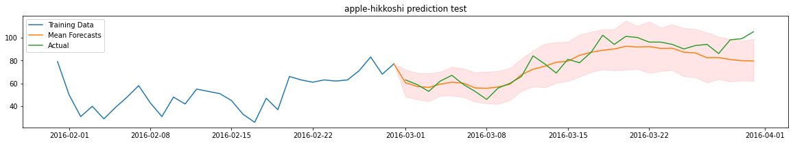
青が学習期間の実数、緑が予測期間の実数、オレンジが予測値になります。それなりに予測出来ているようですが後半は想定より低く予測してしまっているようです。成長企業さまなので年度ごとにプラス補正などしてあげた方がいいのかも知れません。
コンペ提出用に全データで予測モデルを作成
# 環境変数の設定
import os
os.environ['MXNET_USE_FUSION']='0'
%env・・・省略・・・ 'MXNET_USE_FUSION': '0'}
モデル作成中に下記エラーが発生するため設定しています。
ERROR:autogluon.timeseries.trainer: Warning: Exception caused Transformer to fail during training... Skipping this model.
ERROR:autogluon.timeseries.trainer: Traceback (most recent call last):
File "../src/operator/fusion/fused_op.cu", line 672
MXNetError: Check failed: compileResult == NVRTC_SUCCESS (6 vs. 0) : NVRTC Compilation failed. Please set environment variable MXNET_USE_FUSION to 0.
zeros_like_elemwise_addelemwise・・・省略・・・add__mul_scalar__kernel.cu(795): warning: variable "ndim_output0" was declared but never referenced
# https://auto.gluon.ai/stable/api/autogluon.predictor.html#timeseriesdataframe
# データフレームをTimeSeriesDataFrame型に変換
train_data = TimeSeriesDataFrame.from_data_frame(df,timestamp_column="datetime")

# 予測期間 (2016-04-01 ~ 2017-03-31を予測)
prediction_length = 366 # 念のため366日間に設定

!rm -rf autogluon-applehikkoshi_for_competition
# 時系列予測の学習を実施
# https://auto.gluon.ai/stable/api/autogluon.predictor.html#module-5
predictor = TimeSeriesPredictor(
    path="autogluon-applehikkoshi_for_competition",
    target="y", # 目的変数
    prediction_length=prediction_length,
    eval_metric="RMSE"
)

predictor.fit(train_data=train_data,presets="medium_quality")
INFO:autogluon.timeseries.learner:Learner random seed set to 0
INFO:autogluon.timeseries.predictor:presets is set to medium_quality
INFO:autogluon.timeseries.predictor:================ TimeSeriesPredictor ================
INFO:autogluon.timeseries.predictor:TimeSeriesPredictor.fit() called
INFO:autogluon.timeseries.predictor:Setting presets to: medium_quality
INFO:autogluon.timeseries.predictor:Fitting with arguments:
INFO:autogluon.timeseries.predictor:{'evaluation_metric': 'RMSE',
 'hyperparameter_tune_kwargs': None,
 'hyperparameters': 'default',
 'prediction_length': 366,
 'target_column': 'y',
 'time_limit': None}
INFO:autogluon.timeseries.predictor:Provided training data set with 2101 rows, 1 items. Average time series length is 2101.0.
INFO:autogluon.timeseries.predictor:Training artifacts will be saved to: /content/autogluon-applehikkoshi_for_competition
・・・省略・・・
INFO:autogluon.timeseries.trainer:Training complete. Models trained: ['AutoETS', 'ARIMA', 'SimpleFeedForward', 'DeepAR', 'Transformer', 'WeightedEnsemble']
INFO:autogluon.timeseries.trainer:Total runtime: 6852.58 s
INFO:autogluon.timeseries.trainer:Best model: WeightedEnsemble
INFO:autogluon.timeseries.trainer:Best model score: -9.6058
約2時間かかりました。途中GPUのリソースをColab側に止められてしまったので翌日にやり直すなどしていました。
ちなみに翌日まで待つ間に、CPUで学習させてみると完了まで8時間ほどかかりました。
GPUの力はすごいですね。
完了まで待ち続けているのが辛かったので私は実行させておいて、完了したら結果をGoogle Driveに保存するようにしました。
# コピーするだけ
!cp -r autogluon-applehikkoshi_for_competition drive/MyDrive/autogluon-applehikkoshi_for_competition
こうすることでランタイムがColabからリセットされていても結果はGoogle Driveに保存されるので永続化されます。(通常ランタイムをリセットされると/content以下に保存していたファイルなどは消えてしまいます。)
Google Driveに保存するためにはGoogle DriveをColabの環境にマウントしておく必要があります。
マウント方法はデータセットをアップロードしたときと同じように、左側のファイルアイコンをクリックしたらパネル上部にGoogle Driveのアイコンがあるので押下してマウント許可するだけになります。

/contentディレクトリ以下にdriveというフォルダが出現したらマウント成功になります。
※ 数年前はもう少し複雑な手順でマウントしていた気がしますがかなり簡略化されて楽になって良かったです。
# (オプション) saveしたモデルをloadする場合はloadメソッドを使う
# 学習した時に指定したフォルダに学習結果が保存されるので必要あれば呼び出す
# predictor = TimeSeriesPredictor.load("autogluon-applehikkoshi_for_competition")

# ベストモデル
predictor.get_model_best()
# 予測データ作成
predictions = predictor.predict(train_data)predictions
mean 0.1 0.2 0.3 0.4 0.5 0.6 0.7 0.8 0.9 item_id timestamp 0 2016-04-01 79.428337 63.254787 70.651039 73.891457 78.300995 80.431305 83.986748 87.036697 89.532326 92.972588 2016-04-02 77.829102 63.619186 69.904701 72.010315 75.273140 79.287437 81.194695 83.284233 86.349609 90.818733 2016-04-03 72.026009 58.798458 64.403503 66.972610 69.630920 71.452202 74.439041 77.225365 82.038887 84.004623 2016-04-04 68.187294 55.253292 59.225758 62.232117 65.994400 68.716225 72.146942 75.028694 77.289597 80.446976 2016-04-05 67.047012 54.106243 58.106880 61.049206 63.577656 66.925957 69.814705 72.696960 75.899704 80.842506 ... ... ... ... ... ... ... ... ... ... ... 2017-03-28 80.724205 64.835640 69.296982 74.313217 76.972702 82.110687 85.032143 87.537872 93.091171 97.937935 2017-03-29 79.111717 60.212315 66.059380 73.185402 76.367249 80.487022 83.744781 86.468208 90.327408 98.230423 2017-03-30 78.354187 61.644768 67.439369 70.695038 75.253845 77.536064 79.921791 83.943764 88.536469 95.974556 2017-03-31 80.257889 64.401817 68.529594 72.957703 76.446709 79.419769 82.109390 86.200806 90.059860 100.357849 2017-04-01 72.309319 56.666710 62.942562 66.506561 70.401398 72.910629 75.513405 78.892059 81.909210 89.109200 366 rows × 10 columns
366日分予測するようにしたので、2017-04-01まで予測してしまっています。
最終的にコンペに提出するデータからは除外します。
# 一応Google Driveに結果を保存しておく
predictions.loc[0].to_csv("drive/MyDrive/output.csv")
# 予測結果をグラフで確認
plt.figure(figsize=(20, 3))
ytrue = train_data.loc[0]["y"]
ypred = predictions.loc[0]
ypred.loc[ytrue.index[-1]] = [ytrue[-1]] * 10
ypred = ypred.sort_index()
plt.plot(ytrue[-30:], label="Training Data")
plt.plot(ypred["mean"], label="Mean Forecasts")
plt.fill_between(ypred.index, ypred["0.1"], ypred["0.9"], color="red", alpha=0.1)
plt.title("apple-hikkoshi prediction for competition")
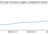
_ = plt.legend()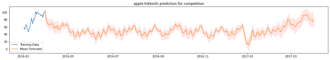
休業日の可能性が高い、年末年始と8/12は0にするなど予測後の調整は必要かもしれません。また、2017-03は2016-3よりも企業自体の規模も大きくなっているでしょうし引っ越し数は上昇傾向にあると思うのでもう少しモデルを工夫する可能性はありそうです。とはいえAutoGluonは日別に長期間の予測もできるので便利ですね。
SIGNATEに予測結果をアップロードする
こちらの記事でターミナルからアップロードする方法をまとめていますのでよろしければご確認ください。
Colabからでも準備すれば出来ると思いますが、今回はGoogle Driveに保存した予測データをローカル環境にコピーしておいたものを加工し提出しようと思います。
Colabでこのままのコードを実行しても動作しないと思うのでご注意ください。
# 予測結果をローカル環境にコピーしたものを読み込む
import pandas as pd
df_result = pd.read_csv("/Users/hinomaruc/Desktop/blog/dataset/applehikkoshi/output.csv")

# 提出用ファイルの作成
df_result.iloc[0:365,0:2].to_csv("applehikkoshi-submission.csv",index=False, header=False)

# 提出
!signate submit --competition-id=269 applehikkoshi-submission.csv --note "model#1 autogluon"You have successfully submitted your predictions.We will send you the submission result to your email address.
評価結果:14.6
残念ながら、結果はあまりよくありませんでした。
まとめ
今回はColabのGPU環境でAutoGluonを使って時系列予測をやってみました。
結果はあまりよくありませんでしたが、AutoMLに組み込まれている時系列モデルの理解が深まったので良しとします。
次回はProphetを試してみたいと思います。
ライブラリのバージョン
autogluon==0.5.2