(その3-3) アップル引越しの需要予測を自己回帰(AR)モデルでやってみた

やっと22年9月の最初の記事を投稿できます。

2週間くらい時系列モデルについて勉強していました。以前も取り組んだことはあるのですが、ARIMAモデルを動かした程度で終わってしまったので今回はもう少し時間をかけてみました。

定常性とかホワイトノイズとか時系列だからこそのワードが出てきて面白かったです。

時系列モデルだけでも下記のような種類があるようです。

1. AR (自己回帰モデル)
2. MA (移動平均モデル)
3. ARMA (自己回帰移動平均モデル)
4. ARIMA (自己回帰和分移動平均モデル)
5. ARIMAX (自己回帰和分移動平均モデル with 外因性変数)
6. Auto ARIMA (自動ARIMAモデル)
7. SARIMA (季節ARIMAモデル)
8. SARIMAX (季節ARIMAモデル with 外因性変数)
9. ARCH (分散自己回帰モデル)
10. GARCH (一般化分散自己回帰モデル)
11. VAR (ベクトル自己回帰モデル)
12. VARMA (ベクトル自己回帰移動平均モデル)

たくさんありますね。

個人的には外因性変数も考慮できるARIMAXやSARIMAXに興味があります。

全部適用できないかも知れませんが、なるべく試してみたいと思います。

それではまずは基本であるARモデルから試してみたいと思います。

※ ARモデルについてはWikipedia参照

自己回帰モデルは、例えば自然科学や経済学において、時間について変動する過程を描写している。（古典的な）自己回帰モデルは実現値となる変数がその変数の過去の値と確率項（確率、つまりその値を完全には予測できない項）に線形に依存している
引用: https://ja.wikipedia.org/wiki/自己回帰モデル

アップル引越しの引越し数をARモデルで予想する

データの読み込み

# アップル引越しのデータセットを読み込む
import pandas as pd
from matplotlib import pyplot as plt
import pandas as pd
# 訓練データと予測付与用データの読み込み
df = pd.read_csv("/Users/hinomaruc/Desktop/blog/dataset/applehikkoshi/train.csv",parse_dates=['datetime'],index_col='datetime')
df_test = pd.read_csv("/Users/hinomaruc/Desktop/blog/dataset/applehikkoshi/test.csv",parse_dates=['datetime'],index_col='datetime')

df.info()

DatetimeIndex: 2101 entries, 2010-07-01 to 2016-03-31
Data columns (total 5 columns):
 #   Column    Non-Null Count  Dtype
---  ------    --------------  -----
 0   y         2101 non-null   int64
 1   client    2101 non-null   int64
 2   close     2101 non-null   int64
 3   price_am  2101 non-null   int64
 4   price_pm  2101 non-null   int64
dtypes: int64(5)
memory usage: 98.5 KB

# 描画設定
from IPython.display import HTML
import seaborn as sns
from matplotlib import ticker
import matplotlib.pyplot as plt
sns.set_style("whitegrid")
from matplotlib import rcParams
rcParams['font.family'] = 'Hiragino Sans' # Macの場合
#rcParams['font.family'] = 'Meiryo' # Windowsの場合
#rcParams['font.family'] = 'VL PGothic' # Linuxの場合
rcParams['xtick.labelsize'] = 12       # x軸のラベルのフォントサイズ
rcParams['ytick.labelsize'] = 12       # y軸のラベルのフォントサイズ
rcParams['axes.labelsize'] = 18        # ラベルのフォントとサイズ
rcParams['figure.figsize'] = 18,8      # 画像サイズの変更(inch)

日付の間隔をasfreqメソッドで変更する

asfreqメソッドはpandasのメソッドで日付の粒度を変更してくれることはもちろん、足りない日付も作成してくれる時系列分析用のデータ作成にとても重宝するメソッドのようです。

# https://pandas.pydata.org/docs/reference/api/pandas.DataFrame.asfreq.html
# 日付の間隔を「日間隔」に変更 (元から日別のデータですが、、週や月間隔にも変更できます)
df = df.asfreq('d')

df.info()

DatetimeIndex: 2101 entries, 2010-07-01 to 2016-03-31
Freq: D
Data columns (total 5 columns):
 #   Column    Non-Null Count  Dtype
---  ------    --------------  -----
 0   y         2101 non-null   int64
 1   client    2101 non-null   int64
 2   close     2101 non-null   int64
 3   price_am  2101 non-null   int64
 4   price_pm  2101 non-null   int64
dtypes: int64(5)
memory usage: 98.5 KB

infoメソッドの返却値にFreq:Dが追加されました。
元々日別データで欠損がないデータなので結果は元データと変更ありません。

わざと欠損日を作成したらどうなるんでしょうか？ちょっと確認してみましょう

(オプション) わざと欠損日を作成したらどうなるか確認

ただの興味本位です。本筋には関係ないので、飛ばしていただいて問題ありません。足りない日付を自動的に埋めて作成してくれるはずです。

df.iloc[5:8]

  

    

      

      
y
      
client
      
close
      
price_am
      
price_pm
    
    

      
datetime
      

      

      

      

      

    
  
  

    

      
2010-07-06
      
14
      
0
      
0
      
-1
      
-1
    
    

      
2010-07-07
      
4
      
0
      
0
      
-1
      
-1
    
    

      
2010-07-08
      
10
      
0
      
0
      
-1
      
-1
    
  

# なんとなく分かりやすいので七夕の日を削除
df_make_nullday = df.drop(index='2010-07-07')

# 削除結果の確認
df_make_nullday.iloc[5:8]

  

    

      

      
y
      
client
      
close
      
price_am
      
price_pm
    
    

      
datetime
      

      

      

      

      

    
  
  

    

      
2010-07-06
      
14
      
0
      
0
      
-1
      
-1
    
    

      
2010-07-08
      
10
      
0
      
0
      
-1
      
-1
    
    

      
2010-07-09
      
12
      
0
      
0
      
-1
      
-1
    
  

七夕である、2010-07-07が削除されていることを確認できました。
この状態でasfreqメソッドを使うとどうなるか確認してみます。

df_make_nullday = df_make_nullday.asfreq('d')
df_make_nullday.iloc[5:8]

  

    

      

      
y
      
client
      
close
      
price_am
      
price_pm
    
    

      
datetime
      

      

      

      

      

    
  
  

    

      
2010-07-06
      
14.0
      
0.0
      
0.0
      
-1.0
      
-1.0
    
    

      
2010-07-07
      
NaN
      
NaN
      
NaN
      
NaN
      
NaN
    
    

      
2010-07-08
      
10.0
      
0.0
      
0.0
      
-1.0
      
-1.0
    
  

2010-07-07の日付データが作成されていますが、NaNのようです。通常であれば欠損値を平均値などで補間してあげる作業が必要になります。

欠損値の確認

df.infoメソッドで確認した通り、欠損値は今回存在しませんのでスキップします。

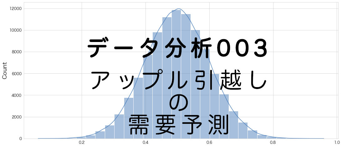
引っ越し数(y)を描画

pandasのplotメソッドで描画できます。

df.y.plot()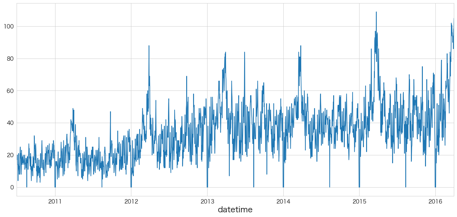

yが正規分布に従うかどうかQQプロットを確認

統計手法を適用するにあたり、おおよそ正規分布を仮定する必要があります。

そのためデータが正規分布に従っているかどうかQQプロットという手法を使って確認します。

# 正規分布に従うかどうかをQQプロットを描画して確認
import scipy.stats as stats
import matplotlib.pyplot as plt

plt.subplot(1,2,1)
sns.histplot(df["y"], kde=True)
plt.subplot(1,2,2)
stats.probplot(df["y"], dist="norm", plot=plt)
plt.show()

左側のグラフがヒストグラム、右側のグラフがQQプロットです。

青い点が赤い線に沿っていれば正規分布であるという表現方法になっています。

端の部分がずれているようですが、なんとなく正規分布に従っていると仮定しようと思います。

もし正規分布に明らかに従っていない場合は対数を取ったりBoxCox変換することによって正規性を担保できる可能性があります。

変数の変換に関してはpower-transform-time-series-forecast-data-pythonの記事が参考になるかと思います。

Mann-Kendall trend検定

まずはデータにトレンドが存在するか存在しないかをテストしてみたいと思います。

次の拡張ディッキー・フラー検定をする時にregressionの設定でtrendを含めるかどうかのオプションがあるので、Mann-Kendall trend検定でtrendが存在するという結果になれば、trendも考慮した拡張ディッキー・フラー検定してみようと思います。

How to Perform a Mann-Kendall Trend Test in Python - Statology

This tutorial explains how to perform a Mann-Kendall trend test in Python, including examples.

www.statology.org

H0: データにトレンドは存在しない
HA: データにトレンドが存在する

でテストをする。

# Mann Kendallのパッケージをインストール
python3 -m pip install pymannkendall

Collecting pymannkendall
  Downloading pymannkendall-1.4.2-py3-none-any.whl (12 kB)
Requirement already satisfied: scipy in ./my-venv/lib/python3.8/site-packages (from pymannkendall) (1.9.1)
Requirement already satisfied: numpy in ./my-venv/lib/python3.8/site-packages (from pymannkendall) (1.23.2)
Installing collected packages: pymannkendall
Successfully installed pymannkendall-1.4.2

# https://pypi.org/project/pymannkendall/
import pymannkendall as mk
mk.original_test(df["y"])

Mann_Kendall_Test(trend='increasing', h=True, p=0.0, z=30.51302505819748, Tau=0.4440819564379774, s=979667.0, var_s=1030826418.3333334, slope=0.016624040920716114, intercept=14.544757033248079)

p <= 0.05なので帰無仮説は棄却され、データにトレンドは存在するという結果になりました。また、trend='increasing'なので上昇トレンドのデータのようです。

そのため、拡張ディッキー・フラー検定ではregression='ct'のオプションを追加しようと思います。

拡張ディッキー・フラー検定で時系列データが(弱)定常か非定常か確認する

帰無仮説と対立仮説は下記になるようです。

H0: 単位根がある
HA: 単位根がない

The null hypothesis of the Augmented Dickey-Fuller is that there is a unit root, with the alternative that there is no unit root. If the pvalue is above a critical size, then we cannot reject that there is a unit root. 引用: https://www.statsmodels.org/dev/generated/statsmodels.tsa.stattools.adfuller.html

時系列データが定常過程か非定常過程かを判断するため、単位根(unit root)があるかどうかを仮説検定するようです。

単位根があると非定常過程、単位根がないと定常過程であるという結論になるようです。

単位根とは？はwikipediaを参照

もし線形な確率過程の特性方程式の根の一つが1であるならば、その確率過程は単位根を持つ。このような確率過程は非定常である。もしこの確率過程の特性方程式の他の根がすべて単位円の内側にあるならば、つまり絶対値が1以下ならば、この確率過程の1階差分は定常である。引用: https://ja.wikipedia.org/wiki/単位根

ちなみに単位根があると自己回帰モデルの傾きを推定する時に「見せかけの回帰」という事象が発生し不安定またはあまり信頼できない結果になる可能性があるようです。

見せかけの回帰は時系列変数の回帰において説明変数と被説明変数が双方とも単位根過程である時に発生しうる。引用:https://ja.wikipedia.org/wiki/見せかけの回帰

見せかけの回帰では、高い決定係数と高いt検定統計量が得られるが、経済学的な意味はまったくない。 引用: https://ja.wikipedia.org/wiki/単位根

そのため、階差や対数変換などにより定常過程にしてから時系列モデルを作成する方が良いようです。

# https://www.statsmodels.org/dev/generated/statsmodels.tsa.stattools.adfuller.html
from statsmodels.tsa.stattools import adfuller

adfuller(df["y"],regression='ct')

(-3.139725669647552,
 0.09709464701226317,
 26,
 2074,
 {'1%': -3.963141667326328,
  '5%': -3.4126089813630323,
  '10%': -3.128297588081566},
 14552.42809850573)

# アウトプットの結果が分かりづらいので、adfullerのヘルプを読む
help(adfuller)

Help on function adfuller in module statsmodels.tsa.stattools:

adfuller(x, maxlag: 'int | None' = None, regression='c', autolag='AIC', store=False, regresults=False)
    Augmented Dickey-Fuller unit root test.

    The Augmented Dickey-Fuller test can be used to test for a unit root in a
    univariate process in the presence of serial correlation.

    Parameters
    ----------
    x : array_like, 1d
        The data series to test.
    maxlag : {None, int}
        Maximum lag which is included in test, default value of
        12*(nobs/100)^{1/4} is used when `None`.
    regression : {"c","ct","ctt","n"}
        Constant and trend order to include in regression.

        * "c" : constant only (default).
        * "ct" : constant and trend.
        * "ctt" : constant, and linear and quadratic trend.
        * "n" : no constant, no trend.

    autolag : {"AIC", "BIC", "t-stat", None}
        Method to use when automatically determining the lag length among the
        values 0, 1, ..., maxlag.

        * If "AIC" (default) or "BIC", then the number of lags is chosen
          to minimize the corresponding information criterion.
        * "t-stat" based choice of maxlag.  Starts with maxlag and drops a
          lag until the t-statistic on the last lag length is significant
          using a 5%-sized test.
        * If None, then the number of included lags is set to maxlag.
    store : bool
        If True, then a result instance is returned additionally to
        the adf statistic. Default is False.
    regresults : bool, optional
        If True, the full regression results are returned. Default is False.

    Returns
    -------
    adf : float
        The test statistic.
    pvalue : float
        MacKinnon's approximate p-value based on MacKinnon (1994, 2010).
    usedlag : int
        The number of lags used.
    nobs : int
        The number of observations used for the ADF regression and calculation
        of the critical values.
    critical values : dict
        Critical values for the test statistic at the 1 %, 5 %, and 10 %
        levels. Based on MacKinnon (2010).
    icbest : float
        The maximized information criterion if autolag is not None.
    resstore : ResultStore, optional
        A dummy class with results attached as attributes.

    Notes
    -----
    The null hypothesis of the Augmented Dickey-Fuller is that there is a unit
    root, with the alternative that there is no unit root. If the pvalue is
    above a critical size, then we cannot reject that there is a unit root.

    The p-values are obtained through regression surface approximation from
    MacKinnon 1994, but using the updated 2010 tables. If the p-value is close
    to significant, then the critical values should be used to judge whether
    to reject the null.

    The autolag option and maxlag for it are described in Greene.

    References
    ----------
    .. [1] W. Green.  "Econometric Analysis," 5th ed., Pearson, 2003.

    .. [2] Hamilton, J.D.  "Time Series Analysis".  Princeton, 1994.

    .. [3] MacKinnon, J.G. 1994.  "Approximate asymptotic distribution functions for
        unit-root and cointegration tests.  `Journal of Business and Economic
        Statistics` 12, 167-76.

    .. [4] MacKinnon, J.G. 2010. "Critical Values for Cointegration Tests."  Queen"s
        University, Dept of Economics, Working Papers.  Available at
        http://ideas.repec.org/p/qed/wpaper/1227.html

    Examples
    --------
    See example notebook

わざわざウェブサイトのAPIを検索しなくていいので便利ですね。

# 検定結果を見やすく加工
result = adfuller(df["y"],regression='ct')
labels = ["検定統計量","P値","#ラグ数","#観測数"]
mod_result = pd.Series(result[0:4],index=labels)
for key,val in result[4].items():
    mod_result[f'臨界値 (有意水準:{key})'] = val;
mod_result

検定統計量               -3.139726
P値                   0.097095
#ラグ数                26.000000
#観測数              2074.000000
臨界値 (有意水準:1%)       -3.963142
臨界値 (有意水準:5%)       -3.412609
臨界値 (有意水準:10%)      -3.128298
dtype: float64

今回の結果ですと、P値が0.05以下ではないため帰無仮説を棄却できず「単位根がないとは言えない」という結果になります。

つまりアップル引っ越しのデータセットは弱定常過程ではなく、非定常過程の可能性がありそうです。

ちなみにP値=0.097は帰無仮説を棄却できない確率が9.7%あるという意味になるようです。これが有意水準以下の値になることによって帰無仮説を棄却することができます。(できない確率という表現だと少し分かりづらいですね)

トレンド・季節性・残差の確認 (seasonal_decompose)

Seasonal decomposition using moving averages.
引用: https://www.statsmodels.org/dev/generated/statsmodels.tsa.seasonal.seasonal_decompose.html

移動平均を使って時系列の分解をしてくれるようです。

from statsmodels.tsa.seasonal import seasonal_decompose
seasonal_decompose(df["y"], model="additive").plot()
plt.show()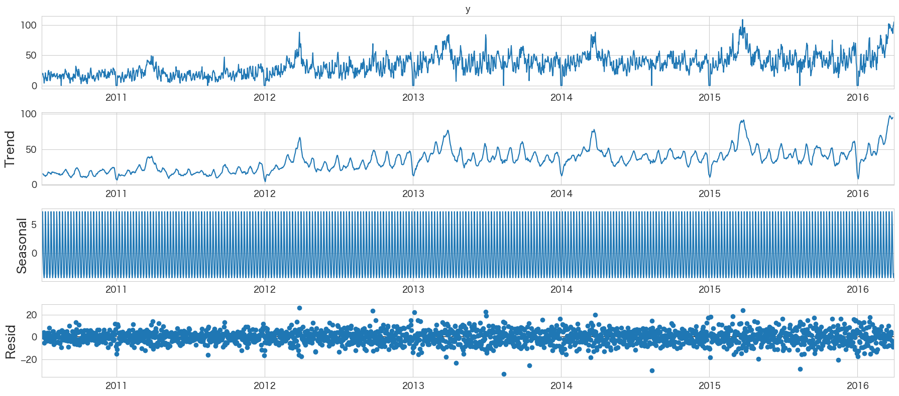

ValueError: Multiplicative seasonality is not appropriate for zero and negative values

model="multiplicative"にするとエラーになってしまいました。y=0の値があるためのようです。とりあえずmodel="additive"の結果を確認してみました。

季節成分がよくわからないですが、Trendはなんとなく伸びていることが分かりますね。

トレンド・季節性・残差の確認 (STL分解)

Season-Trend decomposition using LOESS
引用: https://www.statsmodels.org/dev/generated/statsmodels.tsa.seasonal.STL.html

LOESSを使った時系列の分解をしてくれるようです。

ちなみにLOESSとは回帰手法のことのようです。

loess is a regression technique that uses local weighted regression to fit a smooth curve through points in a sequence
引用: https://towardsdatascience.com/stl-decomposition-how-to-do-it-from-scratch-b686711986ec

from statsmodels.tsa.seasonal import STL
res = STL(df["y"]).fit()
res.plot()
plt.show()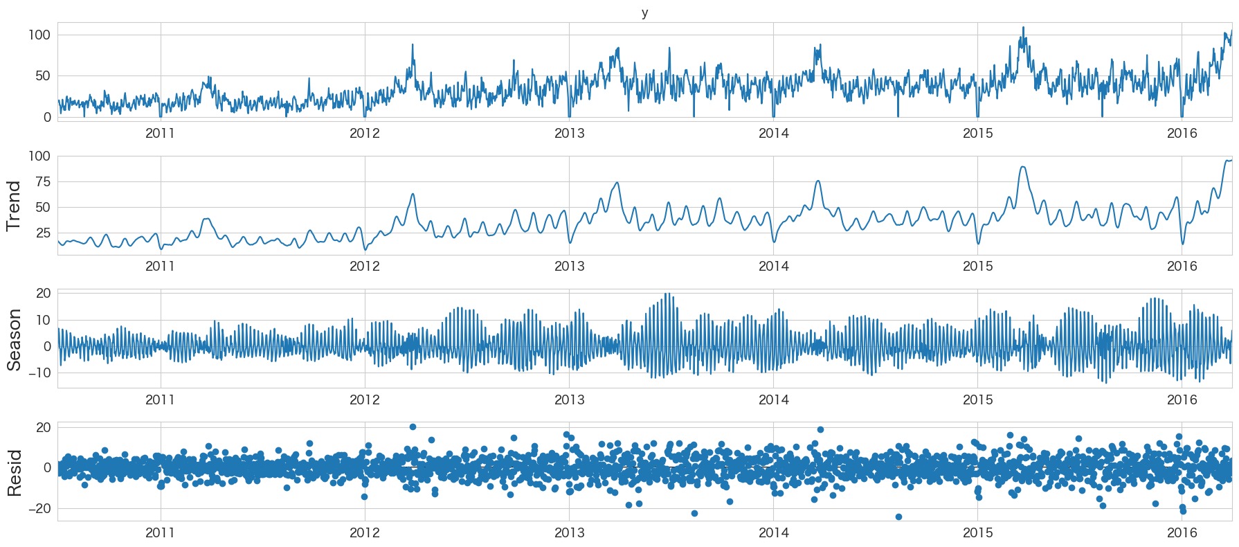

Seasonの見え方がseasonal_decomposeより見やすくなりましたね

自己相関係数の確認

時系列分析において例えば今日の引っ越し数が昨日の引っ越し数と関係があるか、もしくは7日前の引っ越し数と関係があるかといったことを確認できるようです。

statsmodelsのplot_acfメソッドを使って簡単に確認できました。

ModuleNotFoundError: No module named 'statsmodels'

となった場合は、python3 -m pip install statsmodels でライブラリをインストールしてください。

import pandas as pd
import matplotlib.pyplot as plt
from statsmodels.graphics.tsaplots import plot_acf
import numpy as np

fig, ax = plt.subplots(figsize=(16,8))
plot_acf(df['y'], lags=50, zero=False, title="自己相関係数 (autocorrelation)", ax=ax, alpha=0.01)
plt.ylim([0,1])
plt.yticks(np.arange(0.1, 1.1, 0.1))
plt.xticks(np.arange(1, 51, 1))
plt.axhline(y=0.5, color="green")
plt.show()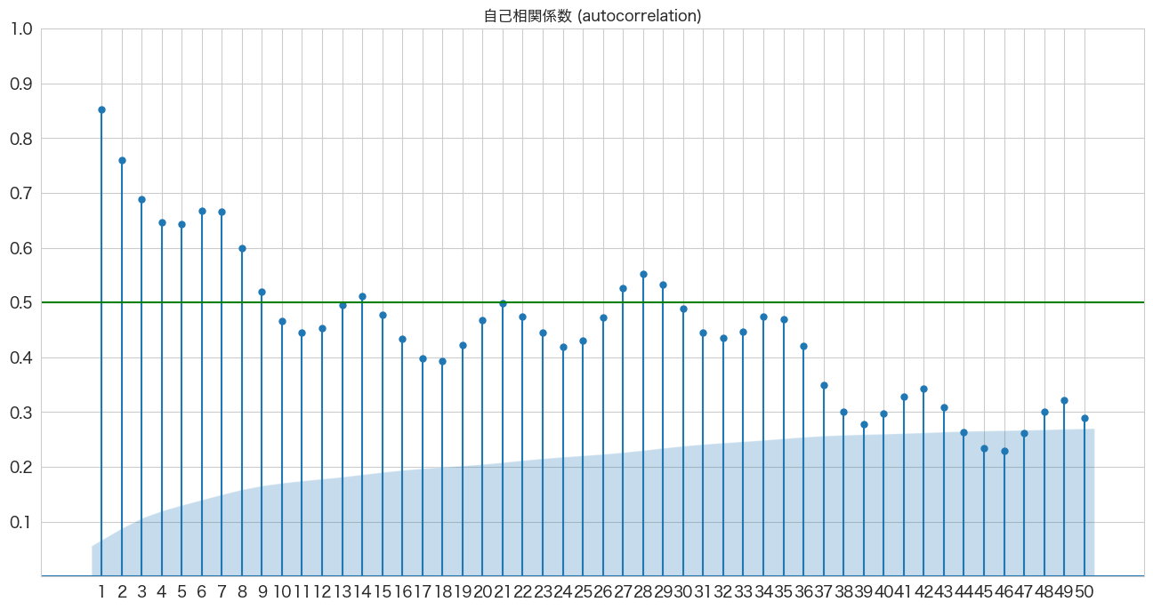

X軸がLag日数で、Y軸が相関係数のようです。

7日前くらい前までは関係ありそうですね。

青いエリアは帰無仮説(H0)が「自己相関係数は0である」の信頼区間のようです(対立仮説は自己相関係数は0ではない)。alpha=0.01で描画したので99%信頼区間を表示してくれているようです。

青いエリア外にプロットがある場合だと帰無仮説は棄却され「自己相関は0ではない」という結論になるようです。

偏自己相関係数の確認

1つ前のトピックで確認した自己相関係数だと今日の引っ越し数と3日前の引っ越し数の自己相関を確認した場合、2日前と1日前の引っ越し数の影響も含まれているようです。偏自己相関係数ではこの2日前と1日前が与える影響を除外した上で3日前の引っ越し数が今日の引っ越し数にどれくらい関係しているかを確認できるようです。

import pandas as pd
import matplotlib.pyplot as plt
from statsmodels.graphics.tsaplots import plot_pacf
import numpy as np

fig, ax = plt.subplots(figsize=(16,8))
plot_pacf(df['y'], lags=50, zero=False, title="偏自己相関係数 (partial autocorrelation)", method=('ywm'), ax=ax, alpha=0.01)
plt.ylim([0,1])
plt.yticks(np.arange(0.1, 1.1, 0.1))
plt.xticks(np.arange(1, 51, 1))
plt.axhline(y=0.5, color="green")
plt.show()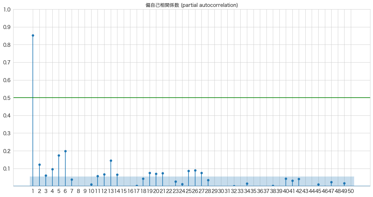

6日前までは青いエリア外にあるので「自己相関は0ではない」と言った結果になりますが、やっぱり今日の引っ越し数は前日の引っ越し数が一番関係していそうですね。ちなみに前日(1日前)の値に関して、自己相関係数と偏自己相関係数は変わらないようです(間の日数がないから当然でしょうか)

非定常過程のデータを定常過程のデータに変換する (階差)

拡張ディッキー・フラー検定で単位根がないとは言えないという結果になったので、本データセットは非定常過程のデータであると思われます。従って階差によって定常過程のデータに変換してモデルを作成しようと思います。

# 確認用に一度dfの値を出力しておく。
df.head()

  

    

      

      
y
      
client
      
close
      
price_am
      
price_pm
    
    

      
datetime
      

      

      

      

      

    
  
  

    

      
2010-07-01
      
17
      
0
      
0
      
-1
      
-1
    
    

      
2010-07-02
      
18
      
0
      
0
      
-1
      
-1
    
    

      
2010-07-03
      
20
      
0
      
0
      
-1
      
-1
    
    

      
2010-07-04
      
20
      
0
      
0
      
-1
      
-1
    
    

      
2010-07-05
      
14
      
0
      
0
      
-1
      
-1
    
  

# https://pandas.pydata.org/docs/reference/api/pandas.DataFrame.diff.html
# 1階差分を取る
df_diff1 = df.diff(periods=1).dropna()
df_diff1.head()

  

    

      

      
y
      
client
      
close
      
price_am
      
price_pm
    
    

      
datetime
      

      

      

      

      

    
  
  

    

      
2010-07-02
      
1.0
      
0.0
      
0.0
      
0.0
      
0.0
    
    

      
2010-07-03
      
2.0
      
0.0
      
0.0
      
0.0
      
0.0
    
    

      
2010-07-04
      
0.0
      
0.0
      
0.0
      
0.0
      
0.0
    
    

      
2010-07-05
      
-6.0
      
0.0
      
0.0
      
0.0
      
0.0
    
    

      
2010-07-06
      
0.0
      
0.0
      
0.0
      
0.0
      
0.0
    
  

df_diff1.y.plot()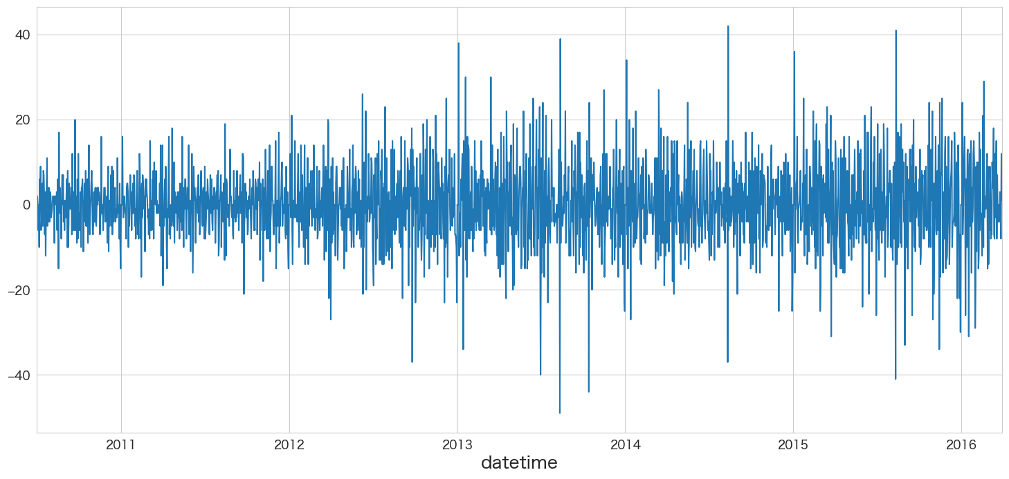

定常過程っぽいデータになりましたね

1.7 ~ 1.12の内容を定常化したデータで確認する

トレンドの検定

# トレンドの検定
import pymannkendall as mk
mk.original_test(df_diff1["y"])

Mann_Kendall_Test(trend='no trend', h=False, p=0.8945870870612784, z=0.13250219489072715, Tau=0.0019283559064407088, s=4250.0, var_s=1028317714.6666666, slope=0.0, intercept=0.0)

「トレンドはあるとは言えない」という結果になりました。

定常性の検定

# 定常性の検定
from statsmodels.tsa.stattools import adfuller
# 検定結果を見やすく加工(今回はトレンドがないので、regression='c'に変更した)
result = adfuller(df_diff1["y"],regression='c')
labels = ["検定統計量","P値","#ラグ数","#観測数"]
mod_result = pd.Series(result[0:4],index=labels)
for key,val in result[4].items():
    mod_result[f'臨界値 (有意水準:{key})'] = val;
mod_result

検定統計量            -1.591158e+01
P値                8.112059e-29
#ラグ数              2.600000e+01
#観測数              2.073000e+03
臨界値 (有意水準:1%)    -3.433508e+00
臨界値 (有意水準:5%)    -2.862935e+00
臨界値 (有意水準:10%)   -2.567513e+00
dtype: float64

P値が0に限りなく近いので帰無仮説が棄却され対立仮説である「単位根がない」と言った結果になりました。単位根がないので非定常過程ではなさそうです。

時系列成分の分解

# 時系列成分の分解
from statsmodels.tsa.seasonal import STL
res = STL(df_diff1["y"]).fit()
res.plot()
plt.show()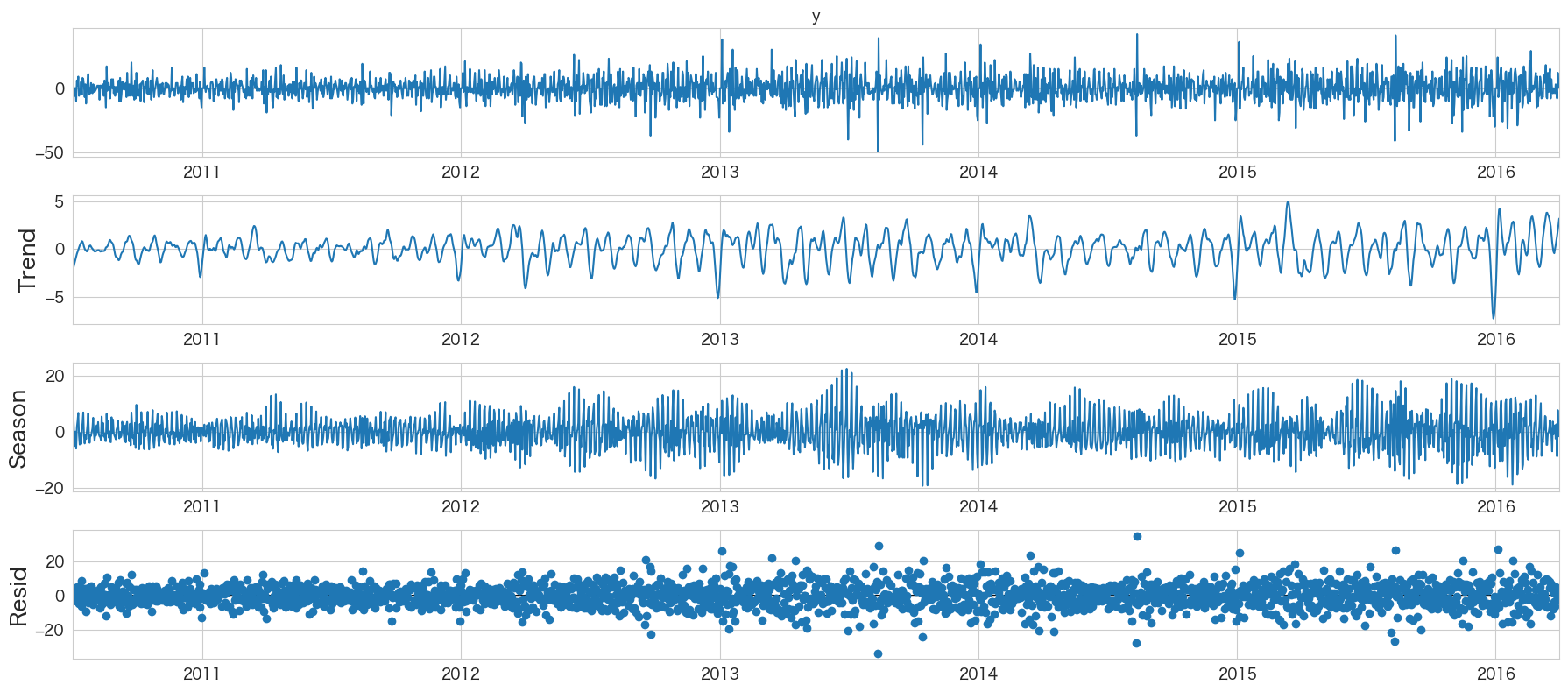

自己相関係数の確認

# 自己相関係数の確認
import pandas as pd
import matplotlib.pyplot as plt
from statsmodels.graphics.tsaplots import plot_acf
import numpy as np

fig, ax = plt.subplots(figsize=(16,8))
plot_acf(df_diff1['y'], lags=50, zero=False, title="自己相関係数 (autocorrelation)", ax=ax, alpha=0.01)
plt.ylim([0,1])
plt.yticks(np.arange(0.1, 1.1, 0.1))
plt.xticks(np.arange(1, 51, 1))
plt.axhline(y=0.5, color="green")
plt.show()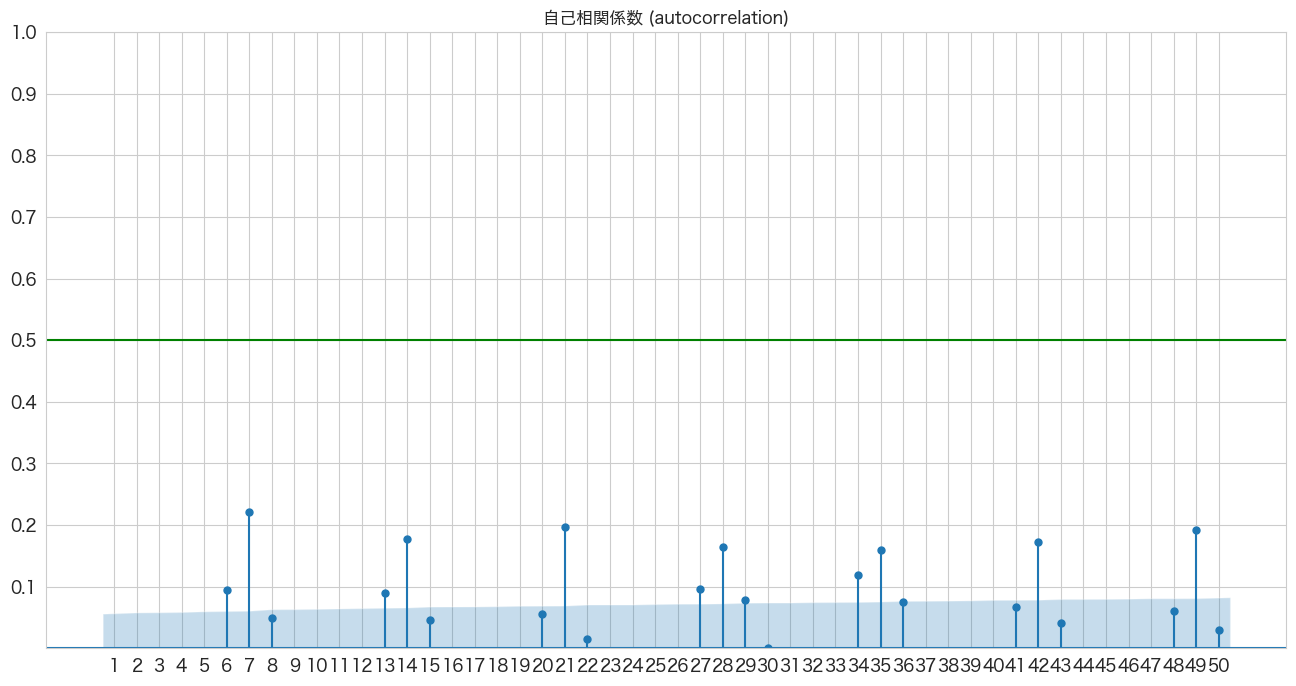

1週間ごとの周期性がありそうですね

偏自己相関係数の確認

# 偏自己相関係数の確認
import pandas as pd
import matplotlib.pyplot as plt
from statsmodels.graphics.tsaplots import plot_pacf
import numpy as np

fig, ax = plt.subplots(figsize=(16,8))
plot_pacf(df_diff1['y'], lags=50, zero=False, title="偏自己相関係数 (partial autocorrelation)", method=('ywm'), ax=ax, alpha=0.01)
plt.ylim([0,1])
plt.yticks(np.arange(0.1, 1.1, 0.1))
plt.xticks(np.arange(1, 51, 1))
plt.axhline(y=0.5, color="green")
plt.show()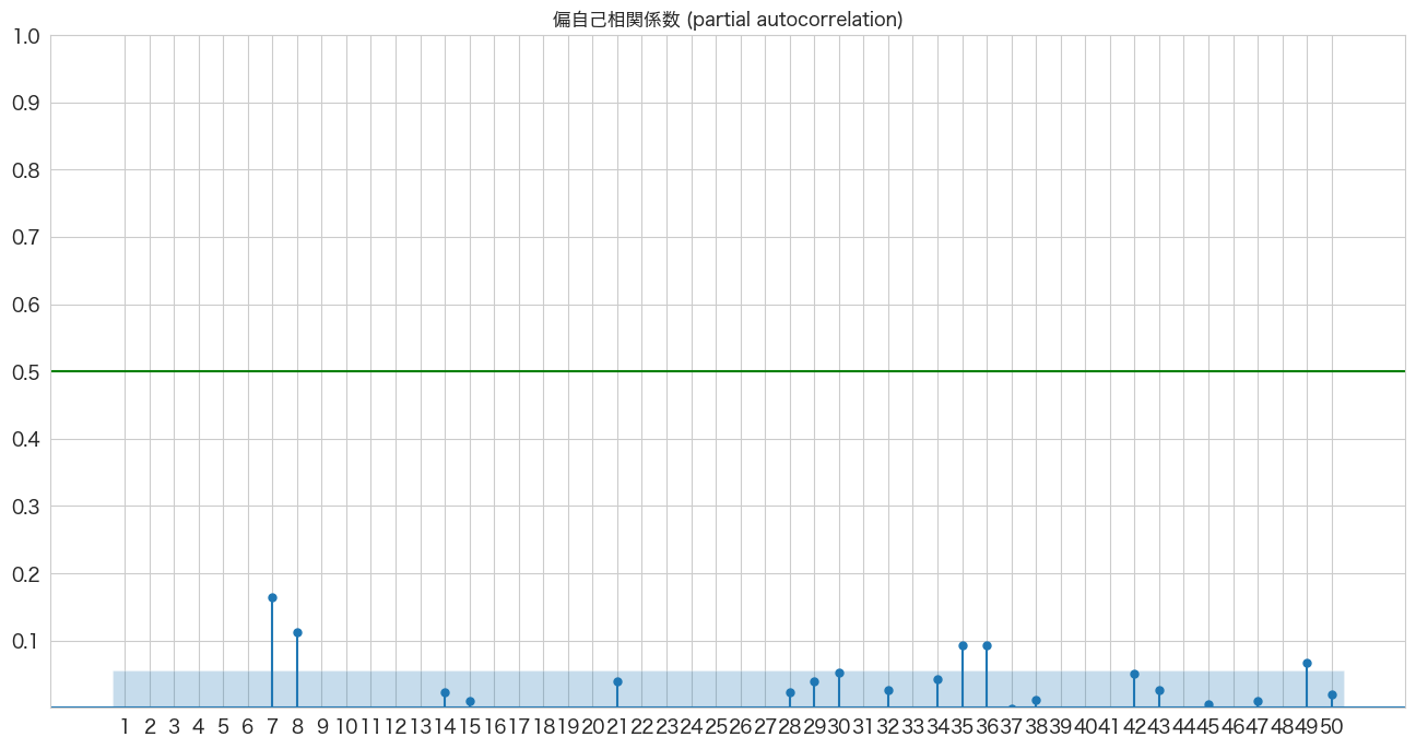

AR(7)、AR(8)、AR(35)、AR(36)らへんが青いエリア外(自己相関は0ではない)にあるようです。

ARモデルの作成

まずは、1次のARモデルy_t=C+ϕ₁y_t-1+ε_tを作成していこうと思います。
一番シンプルな時系列モデルになります。1次からより高次元のARモデルを作成してどの次元(ラグ)のARモデルがいいかは対数尤度比検定(Log likelihood ratio test)で判断すると良いようです。ただし Log likelihoood ratio testは自由度が異なるモデル間を検定するらしく、同じ自由度のモデルを比較する場合はAICやBICを使うようです。

それではARモデルの作成をしていきたいと思います。

from statsmodels.tsa.arima.model import ARIMA
# 1次ARモデルの作成
ar_model = ARIMA(df_diff1["y"],order=(1,0,0))
ret = ar_model.fit()
ret.summary()

SARIMAX Results

  
Dep. Variable:
           
y
        
  No. Observations:  
   
2100
   


  
Model:
            
ARIMA(1, 0, 0)
  
  Log Likelihood     
 
-7637.414


  
Date:
            
Thu, 15 Sep 2022
 
  AIC                
 
15280.829


  
Time:
                
16:42:59
     
  BIC                
 
15297.778


  
Sample:
             
07-02-2010
    
  HQIC               
 
15287.037


  
                   
- 03-31-2016
   
                     
     
 
    


  
Covariance Type:
        
opg
       
                     
     
 
    




     
       
coef
     
std err
      
z
      
P>|z|
  
[0.025
    
0.975]
  


  
const
  
    0.0419
 
    0.169
 
    0.248
 
 0.804
 
   -0.290
 
    0.374


  
ar.L1
  
   -0.1892
 
    0.018
 
  -10.421
 
 0.000
 
   -0.225
 
   -0.154


  
sigma2
 
   84.4613
 
    1.912
 
   44.176
 
 0.000
 
   80.714
 
   88.209




  
Ljung-Box (L1) (Q):
     
0.99
 
  Jarque-Bera (JB):  
 
279.39


  
Prob(Q):
                
0.32
 
  Prob(JB):          
  
0.00
 


  
Heteroskedasticity (H):
 
2.47
 
  Skew:              
  
-0.10


  
Prob(H) (two-sided):
    
0.00
 
  Kurtosis:          
  
4.78
 



Warnings:
[1] Covariance matrix calculated using the outer product of gradients (complex-step).

ar.L1のP>|z|が一次ARモデルのϕ係数の有意性になります。0.05以下なので有意で意味のある係数のようです。

from statsmodels.tsa.arima.model import ARIMA
# 2次ARモデルの作成
ar_model2 = ARIMA(df_diff1["y"],order=(2,0,0))
ret2 = ar_model2.fit()
ret2.summary()

SARIMAX Results

  
Dep. Variable:
           
y
        
  No. Observations:  
   
2100
   


  
Model:
            
ARIMA(2, 0, 0)
  
  Log Likelihood     
 
-7623.602


  
Date:
            
Thu, 15 Sep 2022
 
  AIC                
 
15255.205


  
Time:
                
16:43:08
     
  BIC                
 
15277.803


  
Sample:
             
07-02-2010
    
  HQIC               
 
15263.482


  
                   
- 03-31-2016
   
                     
     
 
    


  
Covariance Type:
        
opg
       
                     
     
 
    




     
       
coef
     
std err
      
z
      
P>|z|
  
[0.025
    
0.975]
  


  
const
  
    0.0410
 
    0.151
 
    0.271
 
 0.786
 
   -0.256
 
    0.338


  
ar.L1
  
   -0.2109
 
    0.018
 
  -11.554
 
 0.000
 
   -0.247
 
   -0.175


  
ar.L2
  
   -0.1142
 
    0.021
 
   -5.383
 
 0.000
 
   -0.156
 
   -0.073


  
sigma2
 
   83.3131
 
    1.900
 
   43.856
 
 0.000
 
   79.590
 
   87.036




  
Ljung-Box (L1) (Q):
     
0.53
 
  Jarque-Bera (JB):  
 
262.93


  
Prob(Q):
                
0.47
 
  Prob(JB):          
  
0.00
 


  
Heteroskedasticity (H):
 
2.49
 
  Skew:              
  
-0.06


  
Prob(H) (two-sided):
    
0.00
 
  Kurtosis:          
  
4.73
 



Warnings:
[1] Covariance matrix calculated using the outer product of gradients (complex-step).

2次ARモデルもar.L1とar.L2はP>|z|が0.05以下なので有意であり意味のある係数のようです。ではAR(1)とAR(2)ではどちらが良いモデルなのでしょうか？
Log Likelihoodは値が大きいほど良く、情報量基準(AIC,BIC,HQIC)は低いほど良いモデルと判断するようです。統計的に2つのモデルに差があるかどうかは対数尤度比検定(Log likelihood ratio test)をしたいと思います。

対数尤度比検定(Log likelihood ratio test)でAR(1)とAR(2)モデルの結果を比較する

# 参考: https://stackoverflow.com/questions/11725115/p-value-from-chi-sq-test-statistic-in-python
LL1 = ret.llf
LL2 = ret2.llf
LLR = 2 * (LL2-LL1)

from scipy.stats.distributions import chi2
p = chi2.sf(LLR,1).round(3)

if p <= 0.05:
    print(f"p値={p}で有意差あり")
else:
    print(f"p値={p}で有意差なし")

p値=0.0で有意差あり

有意差ありなのでAR(2)の方が良いモデルという結果になりました。

このように対数尤度比検定を次数を変えたモデルを適用し、最適なARモデルを探索していこうと思います。

最適な次数のARモデルを求める

# Log likelihood ratio testの関数作成
"""
Log likelihood ratio test
H0: 2つのモデルの比に有意差はない
HA: 2つのモデルの比に有意差がある
引数1: モデル1のLog Likelihood
引数2: モデル2のLog Likelihood
引数3: 自由度
リターン: p値
"""
def llr_test(llf1,llf2,dof):
    LL1 = llf1
    LL2 = llf2
    LLR = 2 * (LL2-LL1)

    from scipy.stats.distributions import chi2
    p = chi2.sf(LLR,dof).round(3)

    return p

# AR(1) ~ AR(40)までで一番良さそうなモデルを探索する。

from statsmodels.tsa.arima.model import ARIMA
import datetime

best_ar_model_fit = None
alpha=0.05

for i in range(1,41):

    # ARモデル作成
    ar_model = ARIMA(df_diff1["y"],order=(i,0,0))
    ar_model_fit = ar_model.fit()

    # AR(1)は自動的にベストモデルになる
    if i == 1:
        best_ar_model_fit = ar_model_fit
    else:
    # AR(2) 以降の処理
        llf1 = best_ar_model_fit.llf
        llf2 = ar_model_fit.llf
        dof = ar_model_fit.model_orders["ar"] - best_ar_model_fit.model_orders["ar"]
        test_result = llr_test(llf1,llf2,dof)

        if test_result <= alpha:
            # 有意差があれば、ベストモデルを更新
            print(f'llr-test result: compare AR({best_ar_model_fit.model_orders["ar"]}) and AR({ar_model_fit.model_orders["ar"]}) -> p値={test_result}')
            best_ar_model_fit = ar_model_fit
            print(f"{datetime.datetime.now()}: best model is AR({i}) -> Log Likelihood:{best_ar_model_fit.llf}、AIC:{best_ar_model_fit.aic}、BIC:{best_ar_model_fit.bic}、HQIC:{best_ar_model_fit.hqic}")
            print("-----")

llr-test result: compare AR(1) and AR(2) -> p値=0.0
2022-09-15 16:44:16.144057: best model is AR(2) -> Log Likelihood:-7623.602345683797、AIC:15255.204691367593、BIC:15277.803461862439、HQIC:15263.482015104586
-----
llr-test result: compare AR(2) and AR(3) -> p値=0.0
2022-09-15 16:44:16.770971: best model is AR(3) -> Log Likelihood:-7603.484685126902、AIC:15216.969370253804、BIC:15245.217833372362、HQIC:15227.316024925047
-----
llr-test result: compare AR(3) and AR(4) -> p値=0.0
2022-09-15 16:44:17.450577: best model is AR(4) -> Log Likelihood:-7554.4190540577、AIC:15120.8381081154、BIC:15154.736263857669、HQIC:15133.25409372089
-----
llr-test result: compare AR(4) and AR(5) -> p値=0.0
2022-09-15 16:44:18.821308: best model is AR(5) -> Log Likelihood:-7497.516611123209、AIC:15009.033222246419、BIC:15048.5810706124、HQIC:15023.518538786158
-----
llr-test result: compare AR(5) and AR(6) -> p値=0.005
2022-09-15 16:44:20.056645: best model is AR(6) -> Log Likelihood:-7493.632382752659、AIC:15003.264765505319、BIC:15048.46230649501、HQIC:15019.819412979306
-----
llr-test result: compare AR(6) and AR(7) -> p値=0.0
2022-09-15 16:44:21.458501: best model is AR(7) -> Log Likelihood:-7465.159327608899、AIC:14948.318655217798、BIC:14999.165888831201、HQIC:14966.942633626033
-----
llr-test result: compare AR(7) and AR(8) -> p値=0.0
2022-09-15 16:44:22.826866: best model is AR(8) -> Log Likelihood:-7451.684345273476、AIC:14923.368690546951、BIC:14979.865616784067、HQIC:14944.061999889436
-----
llr-test result: compare AR(8) and AR(10) -> p値=0.0
2022-09-15 16:44:27.490624: best model is AR(10) -> Log Likelihood:-7441.926083137112、AIC:14907.852166274224、BIC:14975.648477758763、HQIC:14932.684137485205
-----
llr-test result: compare AR(10) and AR(11) -> p値=0.0
2022-09-15 16:44:31.755887: best model is AR(11) -> Log Likelihood:-7432.873992942308、AIC:14891.747985884616、BIC:14965.193989992866、HQIC:14918.649288029847
-----
llr-test result: compare AR(11) and AR(12) -> p値=0.0
2022-09-15 16:44:35.419907: best model is AR(12) -> Log Likelihood:-7403.220241797933、AIC:14834.440483595867、BIC:14913.536180327828、HQIC:14863.411116675345
-----
llr-test result: compare AR(12) and AR(13) -> p値=0.0
2022-09-15 16:44:41.850166: best model is AR(13) -> Log Likelihood:-7394.469243329466、AIC:14818.938486658932、BIC:14903.683876014604、HQIC:14849.978450672657
-----
llr-test result: compare AR(13) and AR(18) -> p値=0.0
2022-09-15 16:45:22.939250: best model is AR(18) -> Log Likelihood:-7382.676943878988、AIC:14805.353887757976、BIC:14918.347740232206、HQIC:14846.740506442944
-----
llr-test result: compare AR(18) and AR(19) -> p値=0.0
2022-09-15 16:45:38.170052: best model is AR(19) -> Log Likelihood:-7375.178153700112、AIC:14792.356307400223、BIC:14910.999852498166、HQIC:14835.812257019441
-----
llr-test result: compare AR(19) and AR(20) -> p値=0.0
2022-09-15 16:45:46.973718: best model is AR(20) -> Log Likelihood:-7367.8567733868895、AIC:14779.713546773779、BIC:14904.006784495432、HQIC:14825.238827327245
-----
llr-test result: compare AR(20) and AR(24) -> p値=0.0
2022-09-15 16:47:02.637493: best model is AR(24) -> Log Likelihood:-7354.508453113671、AIC:14761.016906227342、BIC:14907.90891444384、HQIC:14814.819510517802
-----
llr-test result: compare AR(24) and AR(25) -> p値=0.0
2022-09-15 16:47:23.077121: best model is AR(25) -> Log Likelihood:-7343.9687226566、AIC:14741.9374453132、BIC:14894.479146153411、HQIC:14797.809380537909
-----
llr-test result: compare AR(25) and AR(26) -> p値=0.0
2022-09-15 16:47:46.915367: best model is AR(26) -> Log Likelihood:-7335.745455315361、AIC:14727.490910630722、BIC:14885.682304094644、HQIC:14785.432176789678
-----
llr-test result: compare AR(26) and AR(27) -> p値=0.047
2022-09-15 16:48:22.305341: best model is AR(27) -> Log Likelihood:-7333.777267456277、AIC:14725.554534912553、BIC:14889.395621000187、HQIC:14785.565132005759
-----
llr-test result: compare AR(27) and AR(30) -> p値=0.034
2022-09-15 16:50:28.450351: best model is AR(30) -> Log Likelihood:-7329.454447059043、AIC:14722.908894118085、BIC:14903.699058076854、HQIC:14789.127484014036
-----
llr-test result: compare AR(30) and AR(35) -> p値=0.0
2022-09-15 16:55:01.472330: best model is AR(35) -> Log Likelihood:-7317.22046820731、AIC:14708.44093641462、BIC:14917.479563491946、HQIC:14785.006180981813
-----
llr-test result: compare AR(35) and AR(36) -> p値=0.0
2022-09-15 16:56:01.246234: best model is AR(36) -> Log Likelihood:-7308.229548051409、AIC:14692.459096102819、BIC:14907.147415803856、HQIC:14771.09367160426
-----

# debug
from statsmodels.tsa.arima.model import ARIMA
best_ar_model_fit = ARIMA(df_diff1["y"],order=(36,0,0)).fit()

# ベストモデルのサマリ情報の確認
best_ar_model_fit.summary()

SARIMAX Results

  
Dep. Variable:
           
y
        
  No. Observations:  
   
2100
   


  
Model:
            
ARIMA(36, 0, 0)
 
  Log Likelihood     
 
-7308.230


  
Date:
            
Thu, 15 Sep 2022
 
  AIC                
 
14692.459


  
Time:
                
17:41:28
     
  BIC                
 
14907.147


  
Sample:
             
07-02-2010
    
  HQIC               
 
14771.094


  
                   
- 03-31-2016
   
                     
     
 
    


  
Covariance Type:
        
opg
       
                     
     
 
    




     
       
coef
     
std err
      
z
      
P>|z|
  
[0.025
    
0.975]
  


  
const
  
    0.0387
 
    0.049
 
    0.789
 
 0.430
 
   -0.057
 
    0.135


  
ar.L1
  
   -0.4159
 
    0.018
 
  -23.472
 
 0.000
 
   -0.451
 
   -0.381


  
ar.L2
  
   -0.2603
 
    0.021
 
  -12.203
 
 0.000
 
   -0.302
 
   -0.218


  
ar.L3
  
   -0.1924
 
    0.021
 
   -8.958
 
 0.000
 
   -0.235
 
   -0.150


  
ar.L4
  
   -0.2284
 
    0.021
 
  -10.645
 
 0.000
 
   -0.270
 
   -0.186


  
ar.L5
  
   -0.2313
 
    0.023
 
  -10.245
 
 0.000
 
   -0.276
 
   -0.187


  
ar.L6
  
   -0.1125
 
    0.023
 
   -4.833
 
 0.000
 
   -0.158
 
   -0.067


  
ar.L7
  
    0.0107
 
    0.024
 
    0.454
 
 0.650
 
   -0.035
 
    0.057


  
ar.L8
  
   -0.0583
 
    0.025
 
   -2.367
 
 0.018
 
   -0.107
 
   -0.010


  
ar.L9
  
   -0.1592
 
    0.024
 
   -6.710
 
 0.000
 
   -0.206
 
   -0.113


  
ar.L10
 
   -0.1626
 
    0.024
 
   -6.807
 
 0.000
 
   -0.209
 
   -0.116


  
ar.L11
 
   -0.1597
 
    0.023
 
   -6.800
 
 0.000
 
   -0.206
 
   -0.114


  
ar.L12
 
   -0.2080
 
    0.027
 
   -7.768
 
 0.000
 
   -0.261
 
   -0.156


  
ar.L13
 
   -0.1440
 
    0.026
 
   -5.643
 
 0.000
 
   -0.194
 
   -0.094


  
ar.L14
 
   -0.0696
 
    0.025
 
   -2.763
 
 0.006
 
   -0.119
 
   -0.020


  
ar.L15
 
   -0.0819
 
    0.025
 
   -3.301
 
 0.001
 
   -0.131
 
   -0.033


  
ar.L16
 
   -0.0786
 
    0.026
 
   -3.077
 
 0.002
 
   -0.129
 
   -0.029


  
ar.L17
 
   -0.0886
 
    0.025
 
   -3.485
 
 0.000
 
   -0.138
 
   -0.039


  
ar.L18
 
   -0.1090
 
    0.024
 
   -4.578
 
 0.000
 
   -0.156
 
   -0.062


  
ar.L19
 
   -0.1040
 
    0.025
 
   -4.133
 
 0.000
 
   -0.153
 
   -0.055


  
ar.L20
 
   -0.0933
 
    0.025
 
   -3.796
 
 0.000
 
   -0.141
 
   -0.045


  
ar.L21
 
   -0.0146
 
    0.025
 
   -0.575
 
 0.565
 
   -0.064
 
    0.035


  
ar.L22
 
   -0.0769
 
    0.027
 
   -2.820
 
 0.005
 
   -0.130
 
   -0.023


  
ar.L23
 
   -0.0532
 
    0.027
 
   -1.954
 
 0.051
 
   -0.106
 
    0.000


  
ar.L24
 
   -0.1031
 
    0.026
 
   -4.014
 
 0.000
 
   -0.153
 
   -0.053


  
ar.L25
 
   -0.0840
 
    0.027
 
   -3.152
 
 0.002
 
   -0.136
 
   -0.032


  
ar.L26
 
   -0.0469
 
    0.024
 
   -1.917
 
 0.055
 
   -0.095
 
    0.001


  
ar.L27
 
    0.0048
 
    0.025
 
    0.190
 
 0.849
 
   -0.044
 
    0.054


  
ar.L28
 
    0.0539
 
    0.025
 
    2.120
 
 0.034
 
    0.004
 
    0.104


  
ar.L29
 
    0.0707
 
    0.024
 
    2.961
 
 0.003
 
    0.024
 
    0.117


  
ar.L30
 
    0.0866
 
    0.024
 
    3.606
 
 0.000
 
    0.040
 
    0.134


  
ar.L31
 
    0.0414
 
    0.023
 
    1.792
 
 0.073
 
   -0.004
 
    0.087


  
ar.L32
 
    0.0649
 
    0.024
 
    2.663
 
 0.008
 
    0.017
 
    0.113


  
ar.L33
 
    0.0369
 
    0.023
 
    1.582
 
 0.114
 
   -0.009
 
    0.083


  
ar.L34
 
    0.1040
 
    0.024
 
    4.367
 
 0.000
 
    0.057
 
    0.151


  
ar.L35
 
    0.1312
 
    0.023
 
    5.608
 
 0.000
 
    0.085
 
    0.177


  
ar.L36
 
    0.0927
 
    0.022
 
    4.178
 
 0.000
 
    0.049
 
    0.136


  
sigma2
 
   61.5932
 
    1.509
 
   40.821
 
 0.000
 
   58.636
 
   64.550




  
Ljung-Box (L1) (Q):
     
0.00
 
  Jarque-Bera (JB):  
 
287.41


  
Prob(Q):
                
1.00
 
  Prob(JB):          
  
0.00
 


  
Heteroskedasticity (H):
 
2.24
 
  Skew:              
  
-0.23


  
Prob(H) (two-sided):
    
0.00
 
  Kurtosis:          
  
4.75
 



Warnings:
[1] Covariance matrix calculated using the outer product of gradients (complex-step).

AR(1) ~ AR(40) まで確認をして、AR(36)が良さそうなモデルだという結果になりました。

ar.L36のp値も0.05以下なので有意な係数のようです。また、AICの値もAR(35)より低くなっているので問題なさそうです。今回はAR(36)を採用したいと思います。

この後は予測をして精度確認としたいところですが、作成したモデルが適切かどうか残差分析というものをした方がいいようです。次のセクションでやってみようと思います。

作成したARモデルの残差分析

同志社大学のMingzhe Jin教授のレクチャーノートで勉強させていただきました。Rでの計算例ですが内容が詳しいかつ分かりやすかったです。

作成したモデルの適切さを判断するためには、残差分析が必要である。ARモデルにおける残差は平均0の正規分布に従い、残差の間には相関がないことを期待する。引用: https://mjin.doshisha.ac.jp/R/Chap_34/34.html

残差の正規性はQQプロットで確認することにします。残差の間に相関がない(独立している)ことはBox-Pierce検定とLjung-Box検定を行うと確認できるようです。

resid = best_ar_model_fit.resid
# AR(36)の残差データを確認
resid.plot()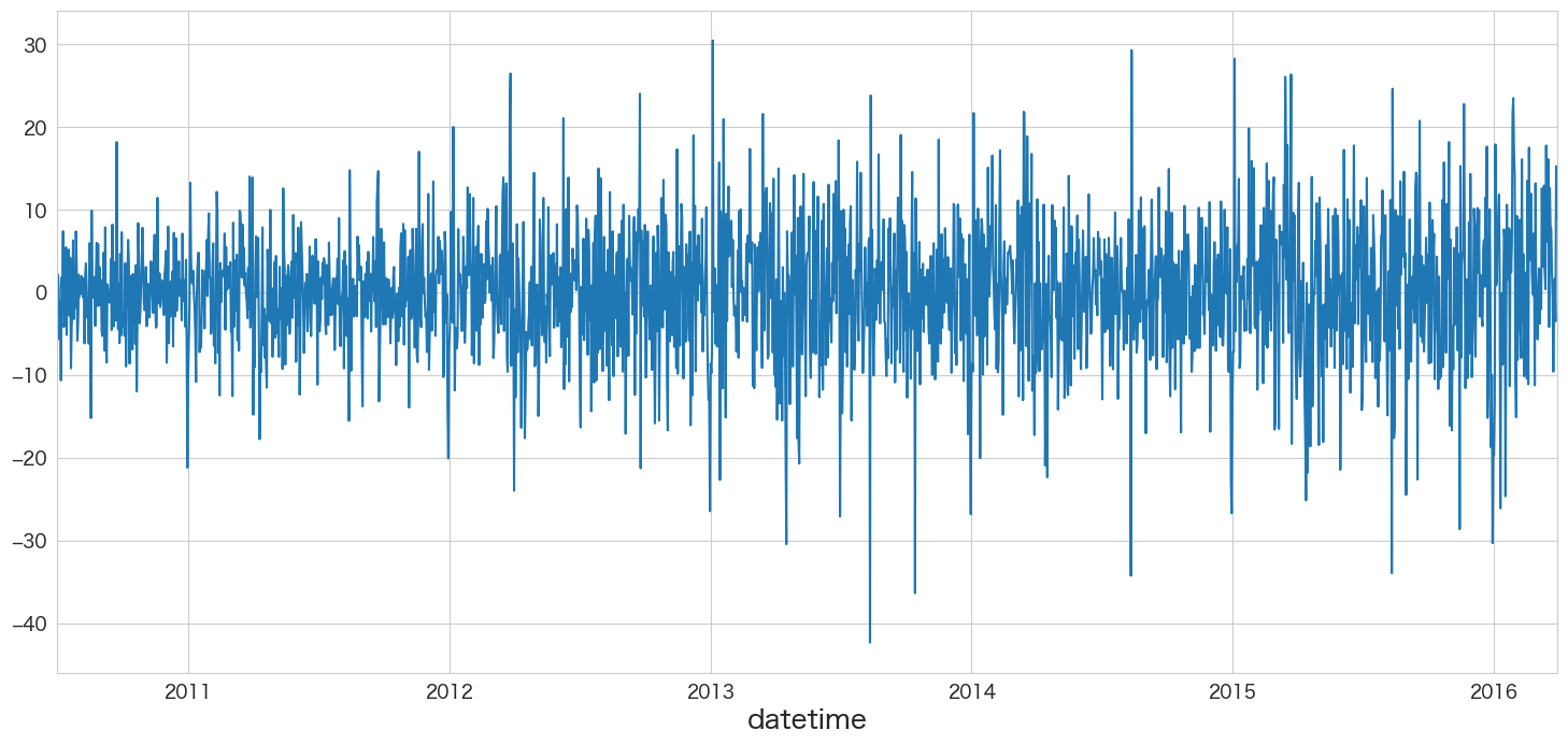

残差の平均と分散を確認

print(f"mean:{resid.mean()}、variance:{resid.var()}")

mean:-0.00247713574697021、variance:61.656562305054244

残差の正規性の確認

# 正規分布に従うかどうかをQQプロットを描画して確認
import scipy.stats as stats
import matplotlib.pyplot as plt

plt.subplot(1,2,1)
sns.histplot(resid, kde=True)
plt.subplot(1,2,2)
stats.probplot(resid, dist="norm", plot=plt)
plt.show()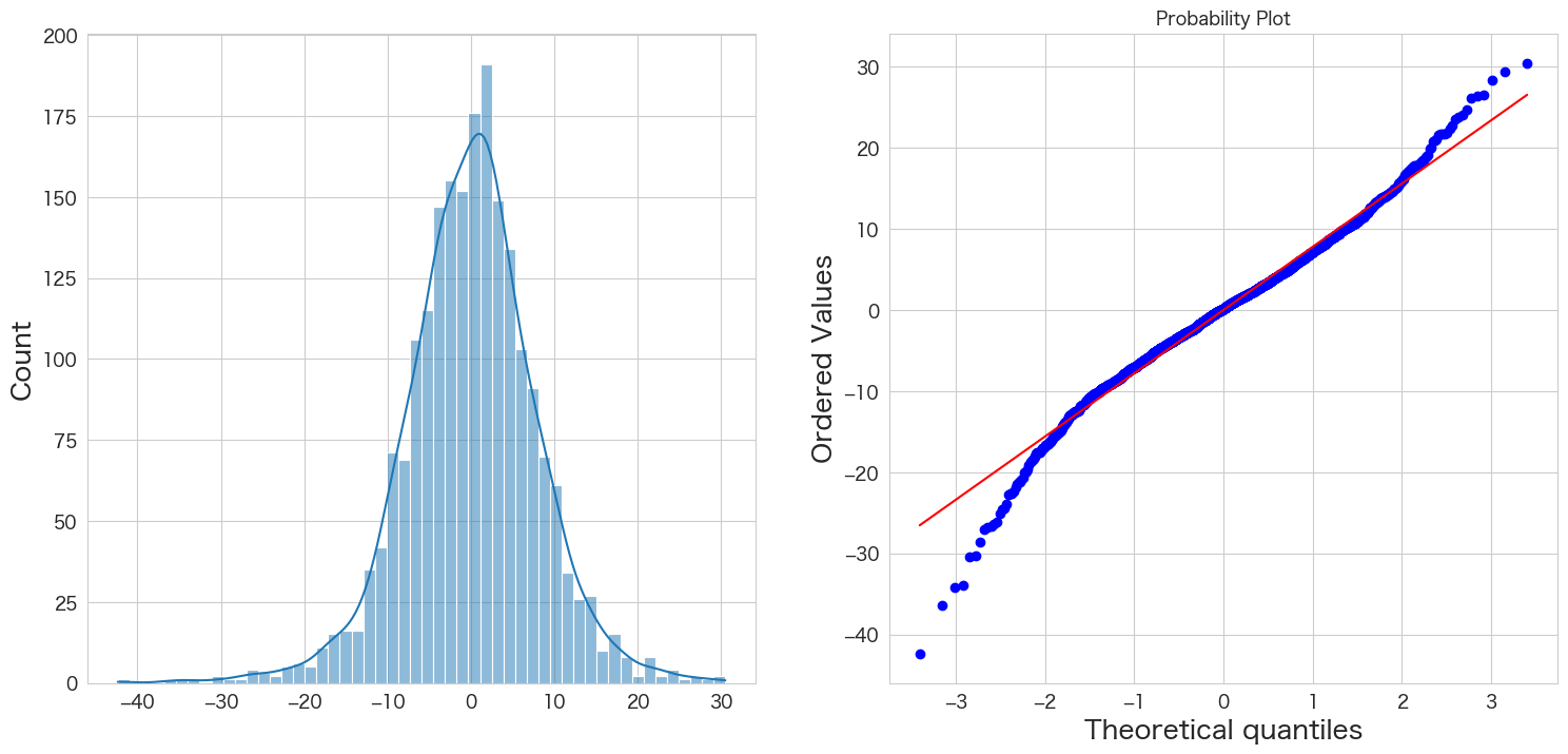

概ね正規分布に従っていそうです。

自己相関係数の確認

# 自己相関係数の確認
import pandas as pd
import matplotlib.pyplot as plt
from statsmodels.graphics.tsaplots import plot_acf
import numpy as np

fig, ax = plt.subplots(figsize=(16,8))
plot_acf(resid, lags=50, zero=False, title="自己相関係数 (autocorrelation)", ax=ax, alpha=0.01)
plt.ylim([0,1])
plt.yticks(np.arange(0.1, 1.1, 0.1))
plt.xticks(np.arange(1, 51, 1))
plt.show()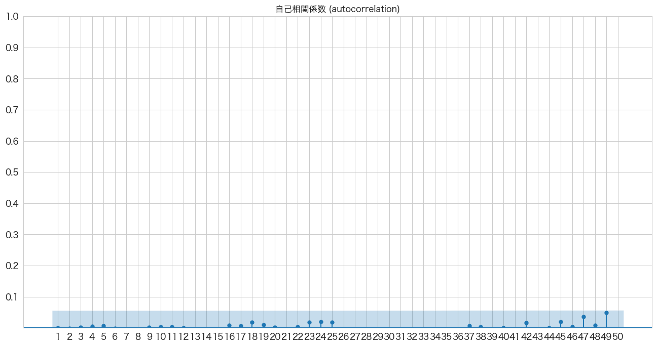

全て青いエリア内なので自己相関はなさそうですね。

Ljung-Box検定で残差の独立性の確認

statsmodelsのacorr_ljungboxでLjung-Box検定とBox-Pierce検定を2つとも出力することが出来るようです。

ただapiの参考情報ではLjung-Box検定の方がよりよい無限サンプルのプロパティがあるとのことなので、Ljung-Box検定を試してみたいと思います。無限サンプルのプロパティとはどういうことでしょうか？結果がインフィニティになり得るということのなのかLjung-Box検定はデータサンプル数が多くてもより正確な結果が期待できるということでしょうか？どちらにせよLung-Box検定を試してみたいと思います　笑

Ljung-Box and Box-Pierce statistic differ in their scaling of the autocorrelation function. Ljung-Box test is has better finite-sample properties. 引用: https://www.statsmodels.org/stable/generated/statsmodels.stats.diagnostic.acorr_ljungbox.html

ちなみに仮説は下記になるようです。

H0: 残差は独立分布している
HA: 残差は独立分布ではない

残差が独立分布していることが望ましいので帰無仮説を棄却しない(P値 >= 0.05)結果になることを期待したいと思います。

# https://www.statsmodels.org/stable/generated/statsmodels.stats.diagnostic.acorr_ljungbox.html

import statsmodels.api as sm
sm.stats.acorr_ljungbox(resid,lags=50)

  

    

      

      
lb_stat
      
lb_pvalue
    
  
  

    

      
1
      
0.000011
      
0.997302
    
    

      
2
      
0.001811
      
0.999095
    
    

      
3
      
0.015038
      
0.999512
    
    

      
4
      
0.081823
      
0.999186
    
    

      
5
      
0.173144
      
0.999376
    
    

      
6
      
0.180821
      
0.999885
    
    

      
7
      
0.231953
      
0.999958
    
    

      
8
      
0.274486
      
0.999987
    
    

      
9
      
0.283389
      
0.999997
    
    

      
10
      
0.316387
      
0.999999
    
    

      
11
      
0.353969
      
1.000000
    
    

      
12
      
0.354114
      
1.000000
    
    

      
13
      
0.647577
      
1.000000
    
    

      
14
      
1.044282
      
0.999999
    
    

      
15
      
1.192962
      
0.999999
    
    

      
16
      
1.329155
      
0.999999
    
    

      
17
      
1.422670
      
1.000000
    
    

      
18
      
2.166647
      
0.999998
    
    

      
19
      
2.396481
      
0.999998
    
    

      
20
      
2.405285
      
0.999999
    
    

      
21
      
2.441820
      
1.000000
    
    

      
22
      
2.474288
      
1.000000
    
    

      
23
      
3.165905
      
1.000000
    
    

      
24
      
3.964076
      
0.999999
    
    

      
25
      
4.639454
      
0.999997
    
    

      
26
      
4.709555
      
0.999999
    
    

      
27
      
5.462359
      
0.999997
    
    

      
28
      
7.666610
      
0.999951
    
    

      
29
      
8.928807
      
0.999874
    
    

      
30
      
9.019655
      
0.999925
    
    

      
31
      
9.107895
      
0.999955
    
    

      
32
      
9.126984
      
0.999976
    
    

      
33
      
9.312103
      
0.999984
    
    

      
34
      
11.481003
      
0.999895
    
    

      
35
      
16.217993
      
0.997190
    
    

      
36
      
18.086110
      
0.994426
    
    

      
37
      
18.213285
      
0.995924
    
    

      
38
      
18.255782
      
0.997179
    
    

      
39
      
20.379741
      
0.993924
    
    

      
40
      
20.379741
      
0.995774
    
    

      
41
      
20.448659
      
0.996982
    
    

      
42
      
21.088891
      
0.997076
    
    

      
43
      
21.387555
      
0.997642
    
    

      
44
      
21.387898
      
0.998393
    
    

      
45
      
22.252702
      
0.998229
    
    

      
46
      
22.292805
      
0.998767
    
    

      
47
      
25.125515
      
0.996292
    
    

      
48
      
25.300950
      
0.997144
    
    

      
49
      
30.485200
      
0.982451
    
    

      
50
      
32.682076
      
0.972351
    
  

デフォルトだと1~10のラグで検定してくれるようです。ラグ50まで確認してみましたがどのラグもP値が0.99以上なので帰無仮説を棄却できず残差は独立分布ではないとは言えないという結果になりました。自己相関係数のグラフも前のセクションで確認しているので期待通りの結果です。

残差分析の結果

残差分析の結果は、AR(36)の残差が平均0の正規分布に従い、かつ残差の間には相関がなかったので問題ないという結果になりました。

AR(36)モデルを使って引っ越し数を予測する

やっとここまで来ました。作成したARモデルで引っ越し数を予測したいと思います。

df_test.index[0]

Timestamp('2016-04-01 00:00:00')

# 2016-04-01 ~ 2017-03-31までの階差を予測
best_ar_model_fit.predict(start = df_test.index[0],end = df_test.index[-1]).plot()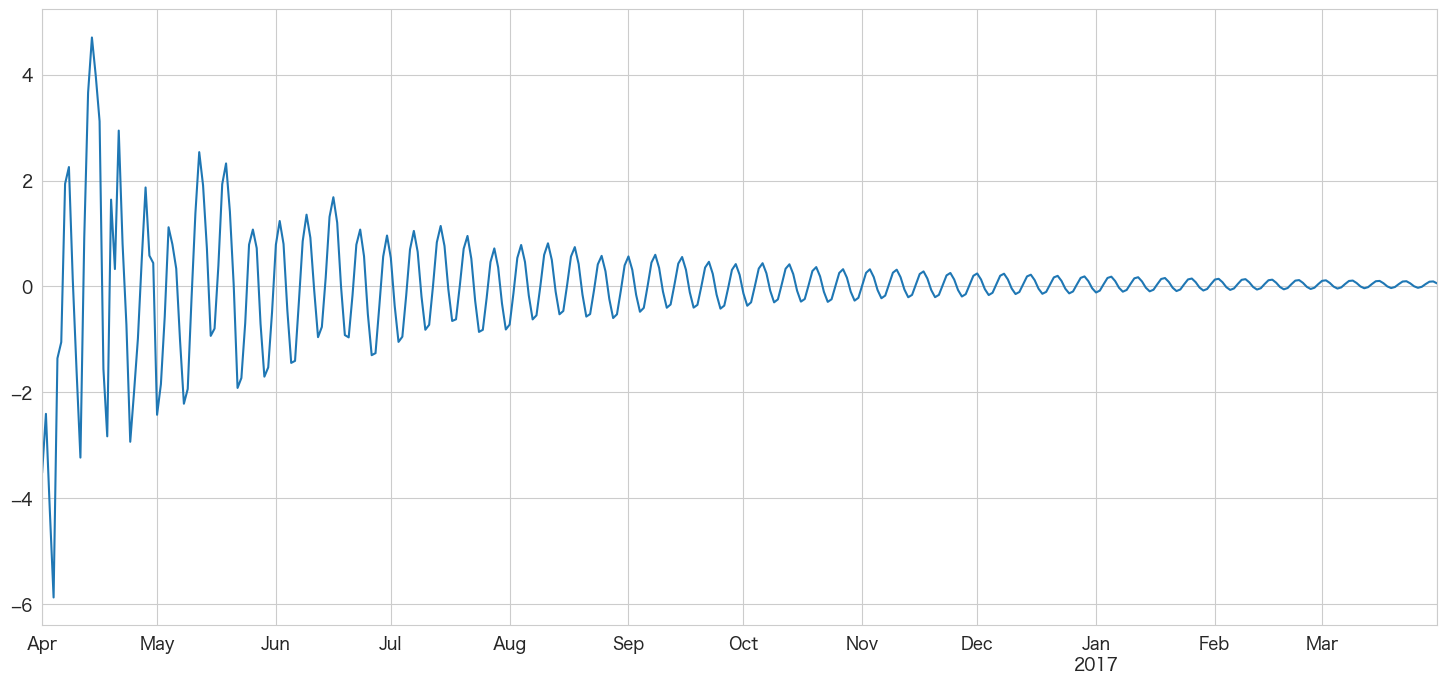

未来の日付が後ろの方になるにつれ予測値が0に近づいてきますね。あまり長い期間の予測には向いていないのかもしれません。月次で12ヶ月先までの予測などに利用した方がいいかも？

上記のグラフは階差の予測なので2016-03-31の引っ越し数から順に足していけば予測値になりそうです。

# 学習データの一番最後の引っ越し数を確認
df.iloc[-1]

y           105
client        1
close         0
price_am      5
price_pm      4
Name: 2016-03-31 00:00:00, dtype: int64

yの値を使います。

predict_diff = best_ar_model_fit.predict(start = df_test.index[0],end = df_test.index[-1])
predict_diff

2016-04-01   -3.520223
2016-04-02   -2.404738
2016-04-03   -4.203624
2016-04-04   -5.872170
2016-04-05   -1.356076
                ...   
2017-03-27   -0.006030
2017-03-28    0.045443
2017-03-29    0.090403
2017-03-30    0.095517
2017-03-31    0.057919
Freq: D, Name: predicted_mean, Length: 365, dtype: float64

y_pred = df.y.iloc[-1]
y_pred_list = []
for idx,val in enumerate(predict_diff):
    y_pred_list.append((y_pred + val))

# テストデータに予測結果を追加
df_test["y_pred"] = y_pred_list

plt.figure(figsize=(20, 3))

ytrue = df.y.iloc[-31:]
ypred = df_test.y_pred

plt.plot(ytrue, label="Training Data")
plt.plot(ypred, label="Forecasts")

plt.title("apple-hikkoshi prediction")
_ = plt.legend()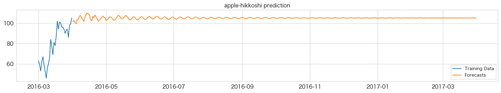

ほとんど横一直線で予測できていなさそうです。以前Wekaという機械学習のツールでARだったかARIMAモデルだったかを試した時も同じような結果になったのを覚えています。これでは予測精度を確認しても意味がないので本記事ではここまでの確認とします。

まとめ

今まで一番長い記事になってしまったかも知れません。時系列分析をきちんとやろうと思うと色々考慮すべき内容があるのですね。

今回の場合、ARモデルでは1年分の日別予測は難しかったようですが勉強できたので個人的には実りある記事となりました。

次はMAモデルを試してみたいと思います。

参考

・https://www.udemy.com/course/time-series-analysis-in-python/
・https://machinelearningmastery.com/power-transform-time-series-forecast-data-python/
・https://www.analyticsvidhya.com/blog/2021/06/statistical-tests-to-check-stationarity-in-time-series-part-1/
・http://www2.hak.hokkyodai.ac.jp/fukuda/lecture/SocialLinguistics/html/07testing.html
・https://researchmap.jp/read0154781/misc/31138386
・https://en.wikipedia.org/wiki/Augmented_Dickey%E2%80%93Fuller_test
・https://bellcurve.jp/statistics/course/9311.html

本記事で利用したライブラリのバージョン

import pandas as pd
import numpy as np
import statsmodels as sm
import matplotlib as mpl
import pymannkendall as mk
import scipy as scp
print('pandas',pd.__version__)
print('numpy',np.__version__)
print('statsmodels',sm.__version__)
print('matplotlib',mpl.__version__)
print('pymannkendall',mk.__version__)
print('scipy',scp.__version__)

pandas 1.4.3
numpy 1.23.2
statsmodels 0.13.2
matplotlib 3.5.3
pymannkendall 1.4.2