今回はAutoGluonというAutoMLライブラリをエイムズのデータセットで試してみます。
MacでAutoMLの環境をする方法は下記記事にまとめています。pipでインストールしているのがほとんどですので、Linuxでも同じようなコードでインストールできるかと思います。
※ brew install しているのは yum や apt に置き換える必要はあります。
(MLJAR) Pythonで3つのAutoML環境を用意してみた
(AutoGluon) Pythonで3つのAutoML環境を用意してみた
(auto-sklearn) Pythonで3つのAutoML環境を用意してみた
それではやってみます。
AutoGluonのアップグレード
なるべく新しいバージョンのライブラリを使うことにします。
source ~/venv-autogluon/bin/activate
(venv-autogluon) python3 -m pip install autogluon --upgradeRequirement already satisfied: autogluon in ./venv-autogluon/lib/python3.8/site-packages (0.4.2) Collecting autogluon Using cached autogluon-0.5.2-py3-none-any.whl (9.6 kB) ・・・省略・・・ Successfully installed Cython-0.29.32 autogluon-0.5.2 autogluon.common-0.5.2 autogluon.core-0.5.2 autogluon.features-0.5.2 autogluon.multimodal-0.5.2 autogluon.tabular-0.5.2 autogluon.text-0.5.2 autogluon.timeseries-0.5.2 autogluon.vision-0.5.2 click-8.0.4 convertdate-2.4.0 distlib-0.3.5 future-0.18.2 gluonts-0.9.7 grpcio-1.43.0 hijri-converter-2.2.4 holidays-0.14.2 hyperopt-0.2.7 korean-lunar-calendar-0.2.1 llvmlite-0.39.0 nlpaug-1.1.10 nltk-3.7 numba-0.56.0 numpy-1.21.6 patsy-0.5.2 platformdirs-2.5.2 pmdarima-1.8.5 protobuf-3.18.1 py4j-0.10.9.5 pymeeus-0.5.11 pytorch-metric-learning-1.3.2 ray-1.13.0 sktime-0.11.4 statsmodels-0.13.2 tbats-1.1.0 tensorboardX-2.5.1 torch-1.11.0 torchtext-0.12.0 torchvision-0.12.0 transformers-4.20.1 virtualenv-20.16.3
バージョン 0.4.2から0.5.2にアップデートされました。
評価指標
住宅IdごとのSalePrice(販売価格)を予測するコンペです。
評価指標は予測SalePriceと実測SalePriceの対数を取ったRoot-Mean-Squared-Error(RMSE)の値のようです。

AutoGluon
分析用データの準備
事前に欠損値処理や特徴量エンジニアリングを実施してデータをエクスポートしています。
本記事と同じ結果にするためには事前に下記記事を確認してデータを用意してください。
(その3-2) エイムズの住宅価格のデータセットのデータ加工①
(その3-3) エイムズの住宅価格のデータセットのデータ加工②
学習用データとスコア付与用データの読み込み
import pandas as pd
import numpy as np
# エイムズの住宅価格のデータセットの訓練データとテストデータを読み込む
df = pd.read_csv("/Users/hinomaruc/Desktop/blog/dataset/ames/ames_train.csv")
df_test = pd.read_csv("/Users/hinomaruc/Desktop/blog/dataset/ames/ames_test.csv")
# 描画設定
import seaborn as sns
from matplotlib import ticker
import matplotlib.pyplot as plt
sns.set_style("whitegrid")
from matplotlib import rcParams
rcParams['font.family'] = 'Hiragino Sans' # Macの場合
#rcParams['font.family'] = 'Meiryo' # Windowsの場合
#rcParams['font.family'] = 'VL PGothic' # Linuxの場合
rcParams['xtick.labelsize'] = 12 # x軸のラベルのフォントサイズ
rcParams['ytick.labelsize'] = 12 # y軸のラベルのフォントサイズ
rcParams['axes.labelsize'] = 18 # ラベルのフォントとサイズ
rcParams['figure.figsize'] = 18,8 # 画像サイズの変更(inch)# 説明変数と目的変数を指定
# 学習データ (AutoGluonは目的変数も含める)
X_train = df.drop(["Id"],axis=1)
# テストデータ
X_test = df_test.drop(["Id"],axis=1)AutoGluonでモデルの作成
# https://auto.gluon.ai/stable/api/autogluon.tabular.TabularPredictor.html
# autogluonのモデル作成
from autogluon.tabular import TabularPredictor
predictor = TabularPredictor(label="SalePrice", problem_type="regression",path="RESULT_AUTOGLUON").fit(X_train, time_limit = 600)
Beginning AutoGluon training ... Time limit = 600s
AutoGluon will save models to "RESULT_AUTOGLUON/"
AutoGluon Version:  0.5.2
Python Version:     3.8.13
Operating System:   Darwin
Train Data Rows:    1460
Train Data Columns: 333
Label Column: SalePrice
Preprocessing data ...
Using Feature Generators to preprocess the data ...
Fitting AutoMLPipelineFeatureGenerator...
    Available Memory:                    9107.26 MB
    Train Data (Original)  Memory Usage: 3.89 MB (0.0% of available memory)
    Inferring data type of each feature based on column values. Set feature_metadata_in to manually specify special dtypes of the features.
    Stage 1 Generators:
        Fitting AsTypeFeatureGenerator...
            Note: Converting 286 features to boolean dtype as they only contain 2 unique values.
    Stage 2 Generators:
        Fitting FillNaFeatureGenerator...
    Stage 3 Generators:
        Fitting IdentityFeatureGenerator...
    Stage 4 Generators:
        Fitting DropUniqueFeatureGenerator...
    Useless Original Features (Count: 7): ['MSSubClass_150', 'YearBuilt_1879', 'YearBuilt_1895', 'YearBuilt_1896', 'YearBuilt_1901', 'YearBuilt_1902', 'YearBuilt_1907']
        These features carry no predictive signal and should be manually investigated.
        This is typically a feature which has the same value for all rows.
        These features do not need to be present at inference time.
    Types of features in original data (raw dtype, special dtypes):
        ('float', []) : 310 | ['LotFrontage', 'LotShape', 'Utilities', 'LandSlope', 'MasVnrArea', ...]
        ('int', [])   :  16 | ['LotArea', 'OverallQual', 'OverallCond', '2ndFlrSF', 'LowQualFinSF', ...]
    Types of features in processed data (raw dtype, special dtypes):
        ('float', [])     :  24 | ['LotFrontage', 'LotShape', 'LandSlope', 'MasVnrArea', 'ExterCond', ...]
        ('int', [])       :  16 | ['LotArea', 'OverallQual', 'OverallCond', '2ndFlrSF', 'LowQualFinSF', ...]
        ('int', ['bool']) : 286 | ['Utilities', 'MSSubClass_120', 'MSSubClass_160', 'MSSubClass_180', 'MSSubClass_190', ...]
    1.0s = Fit runtime
    326 features in original data used to generate 326 features in processed data.
    Train Data (Processed) Memory Usage: 0.88 MB (0.0% of available memory)
Data preprocessing and feature engineering runtime = 1.2s ...
AutoGluon will gauge predictive performance using evaluation metric: 'root_mean_squared_error'
    This metric's sign has been flipped to adhere to being higher_is_better. The metric score can be multiplied by -1 to get the metric value.
    To change this, specify the eval_metric parameter of Predictor()
Automatically generating train/validation split with holdout_frac=0.2, Train Rows: 1168, Val Rows: 292
Fitting 11 L1 models ...
Fitting model: KNeighborsUnif ... Training model for up to 598.8s of the 598.78s of remaining time.
    -49351.2967  = Validation score   (-root_mean_squared_error)
    0.09s    = Training   runtime
    0.07s    = Validation runtime
Fitting model: KNeighborsDist ... Training model for up to 598.59s of the 598.58s of remaining time.
    -49022.574   = Validation score   (-root_mean_squared_error)
    0.06s    = Training   runtime
    0.04s    = Validation runtime
Fitting model: LightGBMXT ... Training model for up to 598.46s of the 598.45s of remaining time.
    -32311.2318  = Validation score   (-root_mean_squared_error)
    2.71s    = Training   runtime
    0.01s    = Validation runtime
Fitting model: LightGBM ... Training model for up to 595.69s of the 595.68s of remaining time.
    -33364.3905  = Validation score   (-root_mean_squared_error)
    0.82s    = Training   runtime
    0.01s    = Validation runtime
Fitting model: RandomForestMSE ... Training model for up to 594.83s of the 594.82s of remaining time.
    -33091.9716  = Validation score   (-root_mean_squared_error)
    4.49s    = Training   runtime
    0.07s    = Validation runtime
Fitting model: CatBoost ... Training model for up to 590.17s of the 590.16s of remaining time.
    -29978.5556  = Validation score   (-root_mean_squared_error)
    21.76s   = Training   runtime
    0.04s    = Validation runtime
Fitting model: ExtraTreesMSE ... Training model for up to 568.35s of the 568.34s of remaining time.
    -32129.1943  = Validation score   (-root_mean_squared_error)
    3.44s    = Training   runtime
    0.07s    = Validation runtime
Fitting model: NeuralNetFastAI ... Training model for up to 564.74s of the 564.72s of remaining time.
No improvement since epoch 3: early stopping
[W ParallelNative.cpp:229] Warning: Cannot set number of intraop threads after parallel work has started or after set_num_threads call when using native parallel backend (function set_num_threads)
    -52385.7488  = Validation score   (-root_mean_squared_error)
    20.07s   = Training   runtime
    0.18s    = Validation runtime
Fitting model: XGBoost ... Training model for up to 544.44s of the 544.43s of remaining time.
    -28249.057   = Validation score   (-root_mean_squared_error)
    4.8s     = Training   runtime
    0.02s    = Validation runtime
Fitting model: NeuralNetTorch ... Training model for up to 539.59s of the 539.58s of remaining time.
[W ParallelNative.cpp:229] Warning: Cannot set number of intraop threads after parallel work has started or after set_num_threads call when using native parallel backend (function set_num_threads)
    -34557.6018  = Validation score   (-root_mean_squared_error)
    5.05s    = Training   runtime
    0.04s    = Validation runtime
Fitting model: LightGBMLarge ... Training model for up to 534.49s of the 534.48s of remaining time.
    -30409.2806  = Validation score   (-root_mean_squared_error)
    2.78s    = Training   runtime
    0.01s    = Validation runtime
Fitting model: WeightedEnsemble_L2 ... Training model for up to 360.0s of the 531.52s of remaining time.
    -27721.2328  = Validation score   (-root_mean_squared_error)
    0.64s    = Training   runtime
    0.0s     = Validation runtime
AutoGluon training complete, total runtime = 69.2s ... Best model: "WeightedEnsemble_L2"
TabularPredictor saved. To load, use: predictor = TabularPredictor.load("RESULT_AUTOGLUON/")
なんか色々自動でやってくれています。
最終的にWeightedEnsembele_L2モデルが選択されたようです。
# 特徴量の重要度の確認
predictor.feature_importance(X_train)
These features in provided data are not utilized by the predictor and will be ignored: ['MSSubClass_150', 'YearBuilt_1879', 'YearBuilt_1895', 'YearBuilt_1896', 'YearBuilt_1901', 'YearBuilt_1902', 'YearBuilt_1907']
Computing feature importance via permutation shuffling for 326 features using 1460 rows with 5 shuffle sets...
1178.64s = Expected runtime (235.73s per shuffle set)
889.07s = Actual runtime (Completed 5 of 5 shuffle sets)
importance
stddev
p_value
n
p99_high
p99_low
TotalLivArea
38261.203832
1094.563494
8.028544e-08
5
40514.925195
36007.482469
OverallQual
23512.093204
936.372603
3.012264e-07
5
25440.097335
21584.089073
BsmtQual
4811.859551
195.716333
3.277030e-07
5
5214.842186
4408.876915
GarageCars
2733.962537
333.895938
2.617385e-05
5
3421.458889
2046.466185
LotArea
2485.904056
60.642905
4.246384e-08
5
2610.768635
2361.039477
...
...
...
...
...
...
...
RoofMatl_CompShg
-2.558456
3.332701
9.194039e-01
5
4.303621
-9.420532
YrSold_2008
-3.084284
4.882976
8.846518e-01
5
6.969831
-13.138400
YearBuilt_1916
-3.790175
2.284067
9.896777e-01
5
0.912750
-8.493101
PoolQC
-36.494475
12.669437
9.985053e-01
5
-10.407929
-62.581021
MoSold_1
-71.427322
47.552748
9.858308e-01
5
26.484442
-169.339086
326 rows × 6 columns
結果がでるまで時間が結構かかりました。
TotalLivAreaとOverallQualが上位に来ているあたり、信用できる結果になっているのかなと思います。
# 自由度調整済みr2を算出
def adjusted_r2(X,Y,Yhat):
    from sklearn.metrics import r2_score
    import numpy as np
    r_squared = r2_score(Y, Yhat)
    adjusted_r2 = 1 - (1-r_squared)*(len(Y)-1)/(len(Y)-X.shape[1]-1)
    return adjusted_r2

# 訓練データへの精度を確認 (オーバーフィット具合を確認する)
print("train r2_adjusted",adjusted_r2(X_train,X_train["SalePrice"], predictor.predict(X_train)))train r2_adjusted 0.9680146829503177
### モデルを適用し、SalePriceの予測をする
df_test["SalePrice"] = predictor.predict(X_train)
df_test[["Id","SalePrice"]]
Id SalePrice 0 1461 208608.531250 1 1462 183918.640625 2 1463 225355.890625 3 1464 141544.953125 4 1465 286628.718750 ... ... ... 1454 2915 187273.500000 1455 2916 173471.203125 1456 2917 208200.875000 1457 2918 266205.906250 1458 2919 142144.937500 1459 rows × 2 columns
# SalePrice(予測) の分布を確認
sns.histplot(df_test["SalePrice"],bins=20)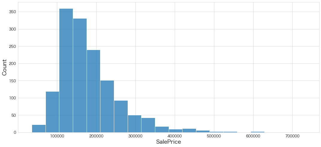
Kaggleにスコア付与結果をアップロード
df_test[["Id","SalePrice"]].to_csv("ames_submission.csv",index=False)!/Users/hinomaruc/Desktop/blog/my-venv/bin/kaggle competitions submit -c house-prices-advanced-regression-techniques -f ames_submission.csv -m "#9 automl autogluon"100%|██████████████████████████████████████| 21.1k/21.1k [00:04<00:00, 5.29kB/s] Successfully submitted to House Prices - Advanced Regression Techniques #9 automl autogluon Score: 0.56305
まさかの全然だめでした。学習時間が足りなかったのかもしれません。600秒にしていたので。。
使用ライブラリのバージョン
pandas Version: 1.3.5
numpy Version: 1.21.6
scikit-learn Version: 1.0.2
seaborn Version: 0.11.2
matplotlib Version: 3.5.2
autogluon Version: 0.5.2
まとめ
次回はautosklearnを試してみたいと思います。